Freon Delivery System (Metric Units)

Summary

This example will model a Freon delivery system to supply Freon at 75 deg. F. As the engineer you will evaluate two candidate refrigerants (Refrigerant 11 and 123) to determine the best choice. We will also calculate the temperature of the hot water supply (i.e., heat exchanger Secondary Fluid) needed for the heat exchangers.

Topics Covered

• Modeling heat transfer

• Entering a resistance curve for a Heat Exchanger

Required Knowledge

This example assumes the user has already worked through the Beginner: Three Reservoir Problem example, or has a level of knowledge consistent with that topic. You can also watch the AFT Fathom Quick Start Video Tutorial Series on the AFT website, as it covers the majority of the topics discussed in the Three-Reservoir Problem example.

Model File

This example uses the following file, which is installed in the Examples folder as part of the AFT Fathom installation:

• US - Freon System with HT.fth

Step 1. Start AFT Fathom

From the Start Menu choose the AFT Fathom 12 folder and select AFT Fathom 12.

To ensure that your results are the same as those presented in this documentation, this example should be run using all default AFT Fathom settings, unless you are specifically instructed to do otherwise.

Step 2. Define the Fluid Properties Group

1. Open Analysis Setup from the toolbar or from the Analysis menu.

2. Open the Fluid panel then define the fluid:

   1. Fluid Library = NIST REFPROP

   2. Fluid = R11 (after selecting, click Add to Model)

   3. Fluid Phase = Liquid

   4. Pressure = 150 psig

   5. Temperature = -50 deg. F

3. Open the Heat Transfer/Variable Fluids panel

   1. Select Heat Transfer With Energy Balance (Single Fluid)

This calculates the default fluid properties to use in the model to initialize the heat transfer calculations.

Note: When Heat Transfer is enabled the fluid properties in the Analysis Setup window are only used as an initial guess. The final fluid properties will be calculated by the Solver.

Step 3. Define the Pipes and Junctions Group

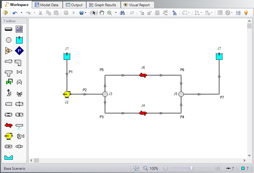
At this point, the first two groups are completed in Analysis Setup. The next undefined group is the Pipes and Junctions group. To define this group, the model needs to be assembled with all pipes and junctions fully defined. Click OK to save and exit Analysis Setup then assemble the model on the workspace as shown in the figure below.

Now enter the properties for the pipes and the junctions.

Pipe Properties

1. Pipe Model tab

   1. Pipe Material = Steel - ANSI

   2. Pipe Geometry = Cylindrical Pipe

   3. Size = 3 inch

   4. Type = STD (schedule 40)

   5. Friction Model Data Set = Standard

   6. Lengths =

Pipe	Length (feet)
1 & 2	10
3 - 6	5
7	30

2. Fittings & Losses tab

   1. P3 - P6 only

      1. Click Specify Fittings & Losses

      2. Bends tab

      3. Standard Threaded, General, 90 deg. (C) Quantity = 1

      4. Click OK

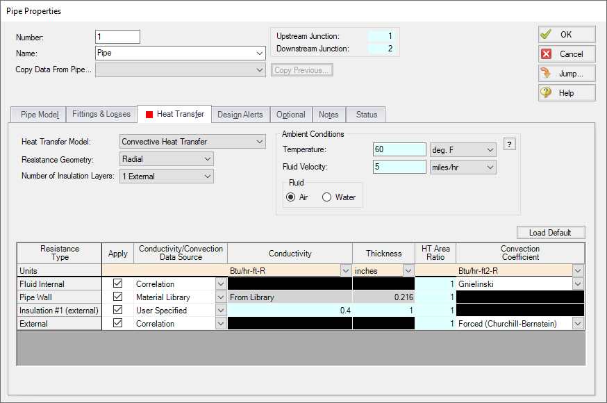
3. Heat Transfer tab (Figure 2)

   1. Heat Transfer Model = Convective Heat Transfer

   2. Resistance Geometry = Radial

   3. Number of Insulation Layers = 1 External

   4. Ambient Conditions

      1. Temperature = 60 deg. F

      2. Fluid Velocity = 5 miles/hr

      3. Fluid = Air

   5. Fluid Internal

      1. Apply = Checked

      2. Conductivity/Convection Data Source = Correlation

      3. HT Area Ratio = 1

      4. Convection Coefficient = Gnielinski

   6. Pipe Wall

      1. Apply = Checked

      2. Conductivity/Convection Data Source = Material Library

      3. Conductivity = From Library

      4. Thickness = 0.216 inches

      5. HT Area Ratio = 1

   7. Insulation #1 (external)

      1. Apply = Checked

      2. Conductivity/Convection Data Source = User Specified

      3. Conductivity = 0.4 Btu/hr-ft-R

      4. Thickness = 1 inches

      5. HT Area Ratio = 1

   8. External

      1. Apply = Checked

      2. Conductivity/Convection Data Source = Correlation

      3. HT Area Ratio = 1

      4. Convection Coefficient = Forced (Churchill-Bernstein)

Junction Properties

1. J1 Reservoir

   1. Name = Supply Reservoir

   2. Liquid Surface Elevation = 10 feet

   3. Liquid Temperature = -50 deg. F

   4. Update Density with Temperature = Checked

   5. Liquid Surface Pressure = 150 psig

   6. Pipe Depth = 0 feet

2. J2 Pump

   1. Inlet Elevation = 2 feet

   2. Pump Model = Centrifugal (Rotodynamic)

   3. Analysis Type = Pump Curve

   4. Enter Curve Data =

Volumetric	Head
gal/min	feet
0	25
200	24
500	15

4. Curve Fit Order = 2

3. J3 & J5 Branches

   1. Elevation = 2 feet

4. J4 & J6 Heat Exchangers

   1. Inlet Elevation = 2 feet

   2. Loss Model tab

      1. Loss Model = Resistance Curve

      2. Enter Curve Data =

Volumetric	Pressure
gal/min	psid
250	2

3. Click Fill As Quadratic

4. Curve Fit Order = 2

5. Click Generate Curve Fit Now

3. Thermal Data tab

   1. Thermal Model = Counter-Flow

   2. Heat Transfer Area = 80 feet2

   3. Overall Heat Transfer Coefficient = 500 Btu/hr-ft-R

   4. Flow Rate = 30 lbm/sec

   5. Specific Heat = 1 Btu/lbm-R

   6. Inlet Temperature = 200 deg. F

Note: This secondary fluid inlet temperature will be the initial guess.

5. J7 Reservoir

   1. Name = Receiving Reservoir

   2. Liquid Surface Elevation = 10 feet

   3. Liquid Temperature = 75 deg. F

   4. Update Density with Temperature = Checked

   5. Liquid Surface Pressure = 150 psig

   6. Pipe Depth = 0 feet

ØTurn on Show Object Status from the View menu to verify if all data is entered. If so, the Pipes and Junctions group in Analysis Setup will have a check mark. If not, the uncompleted pipes or junctions will have their number shown in red. If this happens, go back to the uncompleted pipes or junctions and enter the missing data.

Step 4. Run the Model

Click Run Model on the toolbar or from the Analysis menu. This will open the Solution Progress window. This window allows you to watch as the AFT Fathom solver converges on the answer. This model runs very quickly. Now view the results by clicking the Output button at the bottom of the Solution Progress window.

Step 5. Examine the Output

When the Output is first shown, note that if the default Output Control parameters are being displayed, a warning will be shown stating the HGL, EGL and head loss results may not be meaningful for variable density systems. If all head output parameters are hidden using Output Control, this warning will no longer appear.

Open Output Control by selecting Output Control from the toolbar or Tools menu. Select the Pipes button to display the pipe output parameters, and remove the Head Loss (dH) from the list of shown output by highlighting the parameter and selecting Remove under the table. Next add the Temperature Inlet and Temperature Outlet to the shown output by double-clicking those parameters in the list on the left.

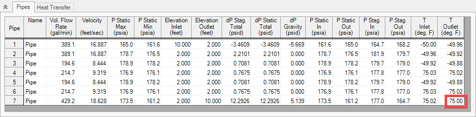
The Output window contains all the data that was specified in the output control window. The output from this model is shown in Figure 3. Now look at the outlet temperature of the last pipe (pipe 7). This is the temperature of the delivered Freon. The temperature is about 115.05 deg. F. This is significantly higher than the required temperature of 75 deg. F.

Now iterate on the temperature of the secondary fluid in the heat exchangers to find the temperature required to produce an outlet temperature of 75.00 deg. F for pipe 7. The answer for this should be 138.5 deg. F. The output for this run in shown in Figure 4.

Now change the fluid on the Fluid panel to R123 and repeat the analysis. For R123, the temperature water supply to the heat exchangers necessary to meet the temperature requirement should be higher, around 154.7 deg. F. If water supply temperature is the main criteria, Refrigerant 11 would be the best choice.