Model Calibration with Pipe Variables - GSC (English Units)
Model Calibration with Pipe Variables - GSC (Metric Units)
Summary
A supply reservoir feeds a water treatment pond through gravity flow and the pipeline has been in existence for about 15 years. The original pipeline delivered about
The objective of this example is to demonstrate how to use the GSC module to determine the amount of additional frictional resistance in the pipeline due to years of corrosion. This could factor into the decision on whether or not to replace the pipeline and when.
For this example, the GSC module will be used to approximate the absolute roughness due to corrosion in the pipeline which has reduced the flow rate from
Note: This example can only be run if you have a license for the GSC module.
Topics Covered
-
Defining the Goal Seek and Control group
-
Setting Variables and Goals
-
Understanding Goal Seek and Control Output
Required Knowledge
This example assumes the user has already worked through the Walk-Through Examples section, and has a level of knowledge consistent with the topics covered there. If this is not the case, please review the Walk-Through Examples, beginning with the Beginner: Three Reservoir Model example. You can also watch the AFT Fathom Quick Start Video Tutorial Series on the AFT website, as it covers the majority of the topics discussed in the Three-Reservoir Model example.
In addition the user should have worked through the Beginner: Heat Transfer in a Pipe - GSC example.
Model File
This example uses the following file, which is installed in the Examples folder as part of the AFT Fathom installation:
Step 1. Start AFT Fathom
From the Start Menu choose the AFT Fathom 12 folder and select AFT Fathom 12.
To ensure that your results are the same as those presented in this documentation, this example should be run using all default AFT Fathom settings, unless you are specifically instructed to do otherwise.
Step 2. Define the Fluid Properties Group
-
Open Analysis Setup from the toolbar or from the Analysis menu.
-
Open the Fluid panel then define the fluid:
-
Fluid Library = AFT Standard
-
Fluid = Water (liquid)
-
After selecting, click Add to Model
-
-
Temperature = 70 deg. F
-
Step 3. Define the Pipes and Junctions Group
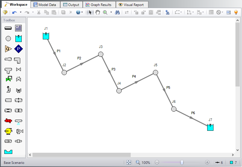
At this point, the first two groups are completed in Analysis Setup. The next undefined group is the Pipes and Junctions group. To define this group, the model needs to be assembled with all pipes and junctions fully defined. Click OK to save and exit Analysis Setup then assemble the model on the workspace as shown in the figure below.
Enter the following pipe and junction properties.
Pipe Properties
-
All Pipes
-
Pipe Material = Steel - ANSI
-
Pipe Geometry = Cylindrical Pipe
-
Size = 8 inch
-
Type = STD (schedule 40)
-
Friction Model Data Set = Standard
-
Length =
| Pipe | Length (feet) |
|---|---|
| 1 & 5 | 5280 |
| 2, 3, & 4 | 2640 |
| 6 | 2000 |
Junction Properties
-
J1 Reservoir
-
Name = Supply Reservoir
-
Liquid Surface Elevation = 1201 feet
-
Liquid Surface pressure = 0 psig
-
Pipe Elevation = 1000 feet
-
-
J2 Branch
-
Elevation = 500 feet
-
-
J3 Branch
-
Elevation = 600 feet
-
-
J4 Branch
-
Elevation = 100 feet
-
-
J5 Branch
-
Elevation = 300 feet
-
-
J6 Branch
-
Elevation = 50 feet
-
-
J7 Reservoir
-
Name = Treatment Pond
-
Liquid Surface Elevation = 10 feet
-
Liquid Surface Pressure = 0 psig
-
Pipe Depth = 0 feet
-
ØTurn on Show Object Status from the View menu to verify if all data is entered. If so, the Pipes and Junctions group in Analysis Setup will have a check mark. If not, the uncompleted pipes or junctions will have their number shown in red. If this happens, go back to the uncompleted pipes or junctions and enter the missing data.
Step 4. Run the Model
Click Run Model on the toolbar or from the Analysis menu. This will open the Solution Progress window. This window allows you to watch as the AFT Fathom solver converges on the answer. This model runs very quickly. Now view the results by clicking the Output button at the bottom of the Solution Progress window.
Step 5. Examine the Output
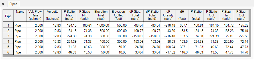
After running the model based upon the original pipeline operation with brand new clean steel pipe, we find that the flow rate is
Step 6. Create a child scenario named Flow Reduction from Corrosion
In the child scenario, we are going to use the GSC module to determine how much additional frictional resistance due to corrosion is in the pipeline. In this new scenario, we know that the flow rate has reduced to
The GSC module is a very useful tool that allows one to calibrate their models so that the predicted results can match measured data. There are four different GSC Pipe Variables that can be used to assist with this calibration including the specified pipe Friction model (i.e., absolute roughness), pipe Design Factor, pipe ID (scaling), and Insulation Thickness.
In order to use GSC to determine the amount of additional frictional resistance due to corrosion, an input parameter must be varied. In this case, we are going to vary each pipe's absolute roughness in order to achieve the desired goal flow rate of
Step 7. Define the Modules Group
Open Analysis Setup, which should bring you to the Modules panel. Check the box next to Activate GSC. The Use option should automatically be selected, making GSC enabled for use.
Step 8. Define the Goal Seek and Control Group
Specify the variables and goals for the model.
Variables Panel
Select the Variables panel within the Goal Seek and Control group. The Variables panel allows users to create and modify the system variables.
In this scenario, we are going to vary the current pipe friction model (i.e., Absolute Roughness) for each pipe in the system. Since there are six individual pipes, there will be six individual pipe variables. If all six variables were to be able to vary independently of each other and there is only one goal associated, then this could lead to a less unique solution (as there could be several different combinations of pipe roughness values that would lead to the desired result). Therefore, we are going to assume that the entire pipeline has the same level of additional frictional resistance due to corrosion. In order to accomplish this, all pipe variables can be linked together. Since only one goal is present, we will only need one effective variable and so all of the pipe variables will be linked to the first variable.
Since there are six pipes, we will set pipes P2 - P6 to be linked to pipe P1.
For pipe P1, set the following variable data:
-
Apply = Selected
-
Object Type = Pipe
-
Junction Type = NA
-
Object Number and Name = P1 (Pipe)
-
Variable Parameter = Friction
-
Link To = (None)
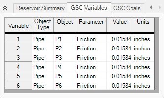
Now, add new variables for pipes P2 - P6. The only differences between the variables for these pipes and the variable for pipe P1 will be the Object Number and Name and instead of selecting (None) under the Link To column, select P1 (Pipe). This will link pipes P2 - P6 to pipe P1 which will force all six pipe variables to be varied identically which requires only one goal to be specified. Figure 3 below shows all the linked pipe variables.
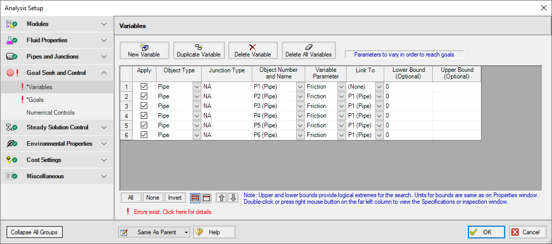
Figure 3: Six pipe variables to vary the pipe friction model (i.e., absolute roughness). Linking all pipes ensures they will be varied identically which makes them effectively one variable.
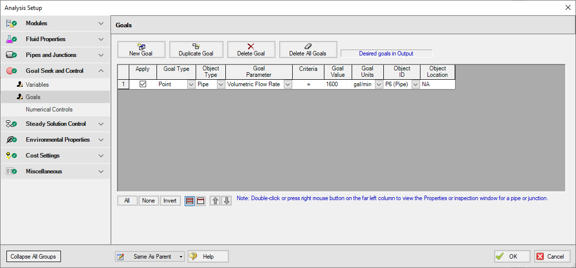
Goals Panel
Goals are the parameter values set by the user that the solver tries to achieve by adjusting the variables. There should be one goal defined for each unlinked variable. Since variables 2 - 6 are all linked to variable 1, only one goal will be required.
Select the Goals panel in the Goal Seek and Control group.
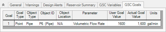
Create a new goal and set up the following goal information:
-
Apply = Selected
-
Goal Type = Point
-
Object Type = Pipe
-
Goal Parameter = Volumetric Flow Rate
-
Criteria = =
-
Goal Value = 1600
-
Goal Units = gal/min
-
Object ID = P6 (Pipe)
-
Object Location = NA
After entering the data, the Goals tab should appear as shown in Figure 4.
On the Numerical Control panel, the Search Method can be modified for Goals between two options, Beta Method and Least Squares. The Beta Method is useful in situations where there are multiple variables and multiple goals. For this model, make sure that the Least Squares method is selected.
Step 9. Run the Model
Click Run Model on the toolbar or from the Analysis menu. This will open the Solution Progress window. This window allows you to watch as the AFT Fathom solver converges on the answer. This model runs very quickly. Now view the results by clicking the Output button at the bottom of the Solution Progress window.
Step 10. Examine the Output
The results of the GSC module analysis are shown in the General section of the Output window. The GSC Variables tab shows the final value for the variable parameter, as shown in Figure 5. The resulting absolute roughness value that would decrease the flow rate to