Heat Exchanger System (English Units)

Heat Exchanger System (Metric Units)

Summary

This example will walk you through a simple calculation to size a pump for a closed loop heat exchanger system. First you will build the system with a fixed flow pump and then enter a pump curve that meets these requirements.

Topics Covered

• Sizing a pump for a specific system

• Entering a loss curve for a Heat exchanger

• Graphing system curves versus pump curves

Required Knowledge

This example assumes the user has already worked through the Beginner: Three Reservoir Problem example, or has a level of knowledge consistent with that topic. You can also watch the AFT Fathom Quick Start Video Tutorial Series on the AFT website, as it covers the majority of the topics discussed in the Three-Reservoir Problem example.

Model File

This example uses the following file, which is installed in the Examples folder as part of the AFT Fathom installation:

• US - Heat Exchanger System.fth

Step 1. Start AFT Fathom

From the Start Menu choose the AFT Fathom 12 folder and select AFT Fathom 12.

To ensure that your results are the same as those presented in this documentation, this example should be run using all default AFT Fathom settings, unless you are specifically instructed to do otherwise.

Step 2. Define the Fluid Properties Group

1. Open Analysis Setup from the toolbar or from the Analysis menu.

2. Open the Fluid panel then define the fluid:

   1. Fluid Library = AFT Standard

   2. Fluid = Water (liquid)

      1. After selecting, click Add to Model

   3. Temperature = 70 deg. F

Step 3. Define the Pipes and Junctions Group

At this point, the first two groups are completed in Analysis Setup. The next undefined group is the Pipes and Junctions group. To define this group, the model needs to be assembled with all pipes and junctions fully defined. Click OK to save and exit Analysis Setup then assemble the model on the workspace as shown in the figure below.

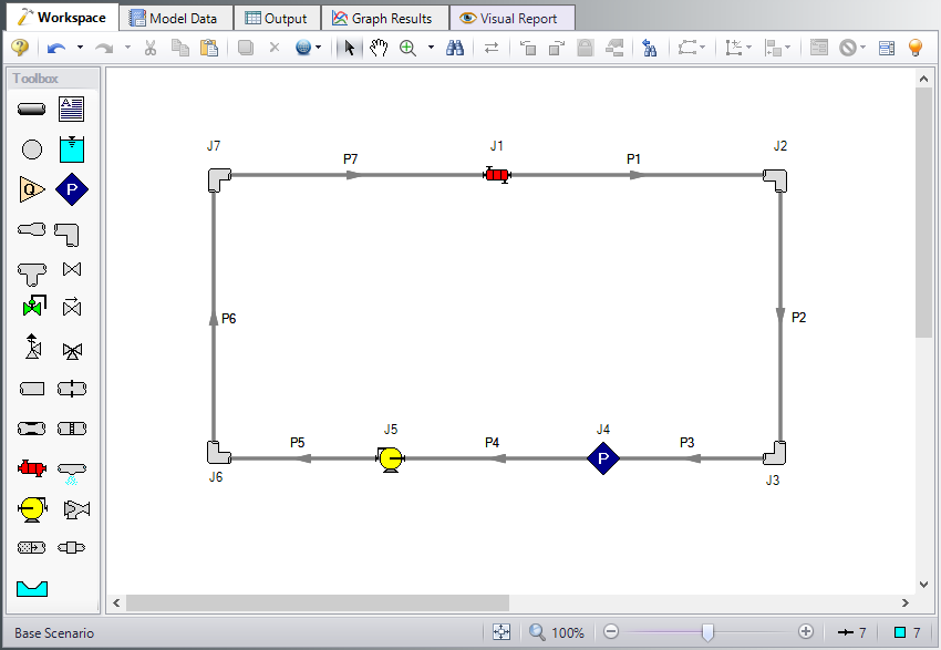
The system is in place but now we need to enter the properties of the objects. Double-click each pipe and junction and enter the following properties. The required information is highlighted in blue.

Pipe Properties

1. Pipe Model tab

   1. Pipe Material = Steel - ANSI

   2. Pipe Geometry = Cylindrical Pipe

   3. Size = 4 inch

   4. Type = STD (schedule 40)

   5. Friction Model Data Set = Standard

   6. Lengths =

Pipe	Length (feet)
1	200
2	15
3	100
4	100
5	200
6	15
7	200

Junction Properties

Specify each junction by entering the following properties in each corresponding Junction Properties window:

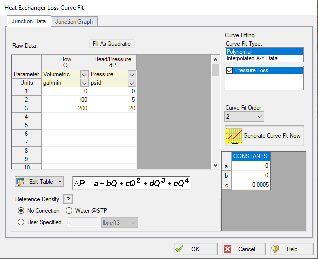
1. J1 Heat Exchanger

   1. Inlet Elevation = 15 feet

   2. Loss Model = Resistance Curve

   3. Enter Curve Data =

Volumetric	Pressure
gal/min	psid
0	0
100	5
200	20

4. Curve Fit Order = 2

5. Click Generate Curve Fit Now

1. J2 & J7 Bend

   1. Inlet Elevation = 15 feet

   2. Type = Standard Elbow (knee, threaded)

   3. Angle = 90 Degrees

2. J3 & J6 Bend

   1. Inlet Elevation = 0 feet

   2. Type = Standard Elbow (knee, threaded)

   3. Angle = 90 Degrees

3. J4 Assigned Pressure

   1. Elevation = 0 feet

   2. Pressure = 100 psia

   3. Pressure Specification = Stagnation

4. J5 Pump

   1. Inlet Elevation = 0 feet

   2. Pump Model = Centrifugal (Rotodynamic)

   3. Analysis Type = Sizing

   4. Parameter = Volumetric Flow Rate

   5. Fixed Flow Rate = 100 gal/min

ØTurn on Show Object Status from the View menu to verify if all data is entered. If so, the Pipes and Junctions group in Analysis Setup will have a check mark. If not, the uncompleted pipes or junctions will have their number shown in red. If this happens, go back to the uncompleted pipes or junctions and enter the missing data.

Step 4. Run the Model

Click Run Model on the toolbar or from the Analysis menu. This will open the Solution Progress window. This window allows you to watch as the AFT Fathom solver converges on the answer. This model runs very quickly. Now view the results by clicking the Output button at the bottom of the Solution Progress window.

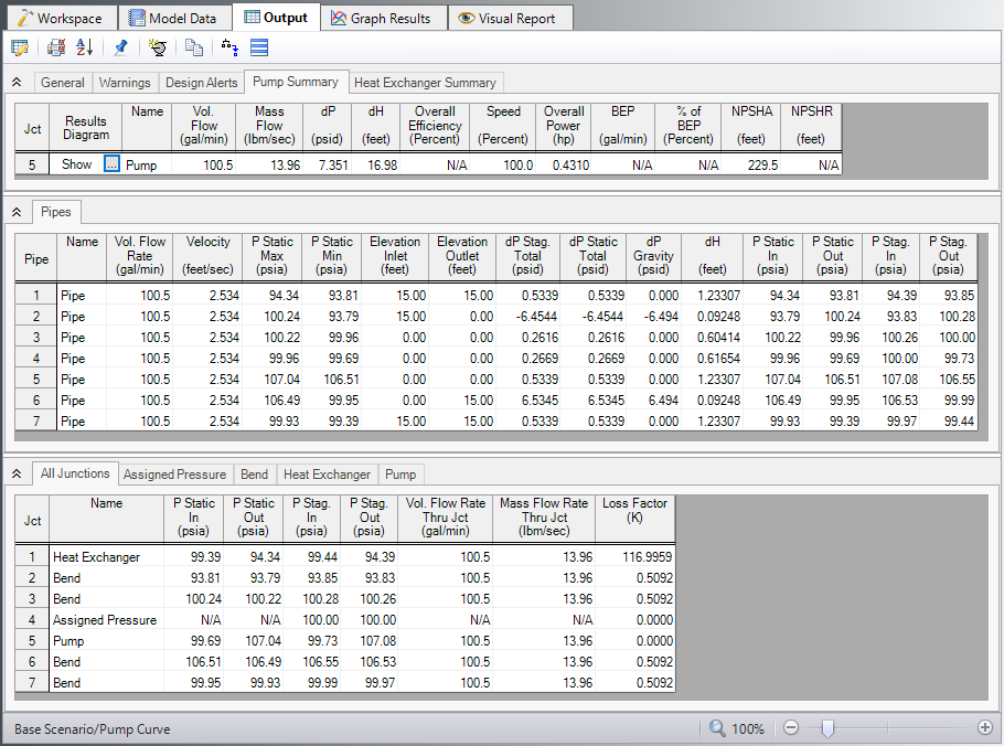
Step 5. Examine the Output

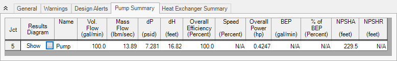
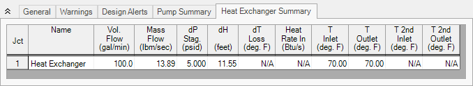
The Output window contains all the data that was specified in the output control window. Because we are interested in the pump requirements for this system, select the Pump Summary tab in the General (top) window. The pump data can also be found in the Junction window (bottom). If we are primarily interested in the head (or pressure) requirement, this is found in the summary window.

For this system, the head requirement of the pump is 7.281 psid (16.82 feet). At the assigned flow rate of 100.0 gal/min, the pressure drop across the heat exchanger was 5.000 psid (11.55 feet) so the total pipe and elbow loss was approximately 2.281 psi (5.27 feet). This output is shown in Figure 3a and Figure 3b.

Step 6. Add Pump Curve

Now that we know the general requirements of the pump, we can select an appropriate pump and enter this data. Open the Pump Properties window and enter the following data:

1. Pump Model = Centrifugal (Rotodynamic)

2. Analysis Type = Pump Curve

3. Enter Curve Data

   1. Flow Q Parameter = Volumetric

   2. Head/Pressure dH Parameter = Head

Volumetric	Head
gal/min	feet
0	20
100	17
200	12

3. Curve Fit Order = 2

4. Click Generate Curve Fit Now

Step 7. Re-evaluate the Model

Select Run Model from the toolbar or Analysis menu. Because the pump head at 100 gal/min was slightly higher than required, the system will adjust with a slightly higher flow rate. The output of this run is shown in Figure 4.

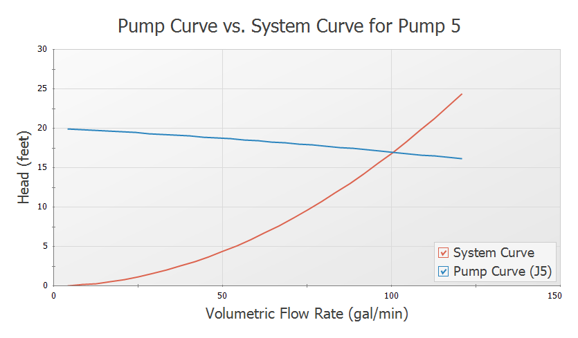
This system is a good example to demonstrate how to use the Graph Results Tab. Change to the Graph Results window by choosing it from the Window drop-down on the menu bar, clicking the Graph Results tab on the toolbar, or by pressing CTRL+G. Now the Graph Control window will be displayed on the Quick Access Panel as shown in Figure 5. Select Pump Curve vs. System Curve and Fathom automatically selects the data you want to graph.

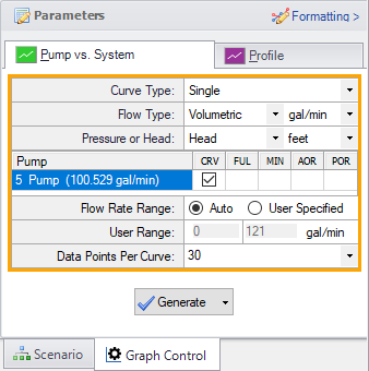
Click Generate to view this graph. This graph is shown in Figure 6. The red line shows the pump curve that we entered. This starts out with 20 feet of head available at 0 gal/min and decreases slowly with increasing flow rate. The blue line is the overall system curve. The head requirement increases significantly with flow rate. Most of the pressure loss (head loss) is through the heat exchanger but this graph also includes the pipe and elbow loss. The lines cross right at 100.5 gal/min which is the operating point shown in the output in Figure 4.