Heat Transfer in a Pipe (Metric Units)

Summary

The objective of this example is to demonstrate how to calculate heat transfer in a pipe. For this example we will specify a mass flow rate and an inlet temperature and calculate the outlet temperature and total heat loss for a 100 foot section of pipe.

Topics Covered

• Modeling heat transfer in a single pipe

Required Knowledge

This example assumes the user has already worked through the Beginner: Three Reservoir Problem example, or has a level of knowledge consistent with that topic. You can also watch the AFT Fathom Quick Start Video Tutorial Series on the AFT website, as it covers the majority of the topics discussed in the Three-Reservoir Problem example.

Model File

This example uses the following file, which is installed in the Examples folder as part of the AFT Fathom installation:

• US - Heat Transfer.fth

Step 1. Start AFT Fathom

From the Start Menu choose the AFT Fathom 12 folder and select AFT Fathom 12.

To ensure that your results are the same as those presented in this documentation, this example should be run using all default AFT Fathom settings, unless you are specifically instructed to do otherwise.

Step 2. Define the Fluid Properties Group

1. Open Analysis Setup from the toolbar or from the Analysis menu.

2. Open the Fluid panel then define the fluid:

   1. Fluid Library = AFT Standard

   2. Fluid = Water (liquid)

      1. After selecting, click Add to Model

   3. Temperature = 70 deg. F

4. This calculates the default fluid properties to use in the model to initialize the heat transfer calculations.

3. Open the Heat Transfer/Variable Fluids panel:

   1. Heat Transfer = Heat Transfer With Energy Balance (Single Fluid)

Step 3. Define the Pipes and Junctions Group

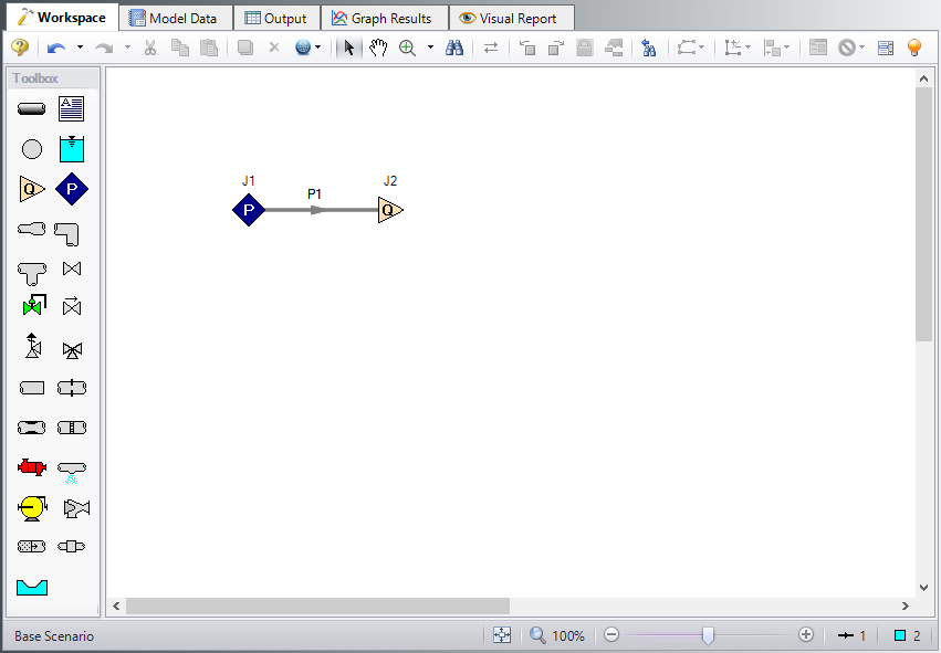
At this point, the first two groups are completed in Analysis Setup. The next undefined group is the Pipes and Junctions group. To define this group, the model needs to be assembled with all pipes and junctions fully defined. Click OK to save and exit Analysis Setup then assemble the model on the workspace as shown in the figure below.

Although one pipe is all that we are modeling, we still need junctions at each end to define the pressure and flow conditions for this pipe.

The system is in place but now we need to enter the properties of the objects. Double-click each pipe and junction and enter the following properties. The required information is highlighted in blue.

Pipe Properties

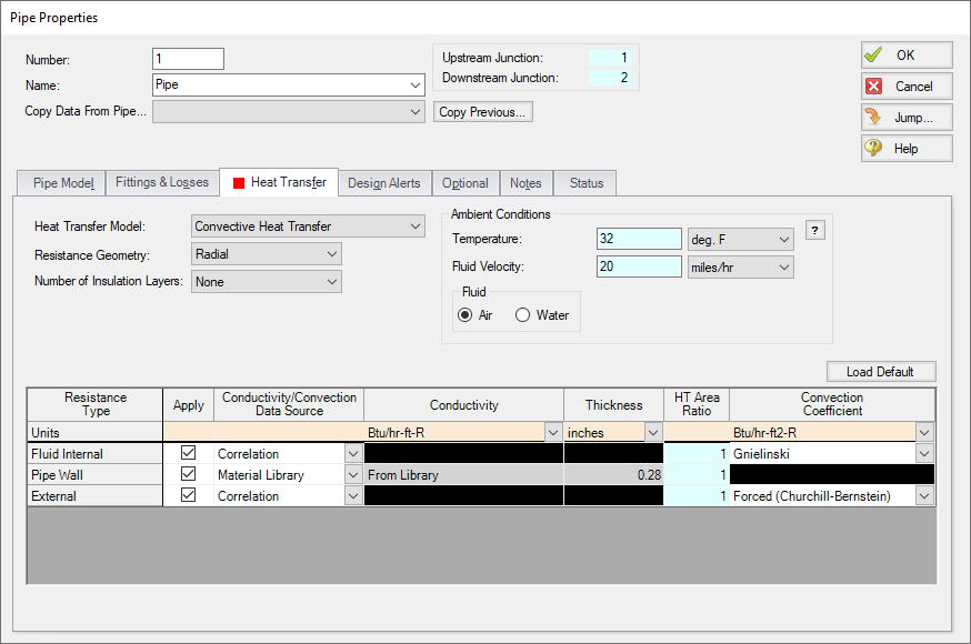
Because heat transfer was selected on the Heat Transfer/Variable Fluids panel in Analysis Setup, the Pipe Properties window has an additional tab to define: Heat Transfer. We will use Convective Heat Transfer for this example. Fathom allows you to perform a layered heat transfer analysis with internal and external convection coefficients and conduction through multiple insulation layers. For this example, we will consider the internal convection, conduction through the pipe wall, and external convection as affecting heat transfer in our system.

Pipe P1

1. Pipe Model tab

   1. Pipe Material = Steel - ANSI

   2. Pipe Geometry = Cylindrical Pipe

   3. Size = 6 inch

   2. Type = STD (schedule 40)

   3. Friction Model Data Set = Standard

   4. Length = 300 feet

2. Heat Transfer tab

   1. Heat Transfer Model = Convective Heat Transfer

   2. Ambient Conditions

      1. Temperature = 32 deg. F

      2. Fluid Velocity = 20 miles/hr

      3. Fluid = Air

   3. Fluid Internal

      1. Apply = Checked

      2. Conductivity/Convection Data Source = Correlation

      3. HT Area Ratio = 1

      4. Convection Coefficient = Gnielinski

   4. Pipe Wall

      1. Apply = Checked

      2. Conductivity/Convection Data Source = Material Library

      3. Conductivity = From Library

      4. Thickness = 0.28 inches

      5. HT Area Ratio = 1

   5. External

      1. Apply = Checked

      2. Conductivity/Convection Data Source = Correlation

      3. HT Area Ratio = 1

      4. Convection Coefficient = Forced (Churchill-Bernstein)

The heat transfer window looks like Figure 2 below.

Junction Properties

Now that the pipe is defined, specify the junction properties:

1. J1 Assigned Pressure

   1. Elevation = 0 feet

   2. Pressure = 50 psia

   3. Temperature = 150 deg. F

   4. Pressure Specification = Stagnation

2. J2 Assigned Flow

   1. Elevation = 0 feet

   2. Type = Outflow

   3. Flow Specification = Mass Flow Rate

   4. Flow Rate = 10 lbm/sec

Note: The temperature at J2 will not be used by Fathom because the outlet temperature is defined by the inlet temperature and the heat loss through the pipe.

ØTurn on Show Object Status from the View menu to verify if all data is entered. If so, the Pipes and Junctions group in Analysis Setup will have a check mark. If not, the uncompleted pipes or junctions will have their number shown in red. If this happens, go back to the uncompleted pipes or junctions and enter the missing data.

Step 4. Run the Model

Click Run Model on the toolbar or from the Analysis menu. This will open the Solution Progress window. This window allows you to watch as the AFT Fathom solver converges on the answer. This model runs very quickly. Now view the results by clicking the Output button at the bottom of the Solution Progress window.

Step 5. Examine the Output

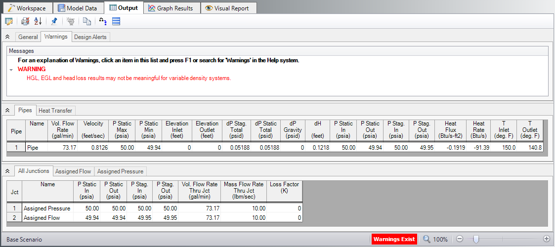
Open the Output Control window by selecting Output Control from the Output toolbar or Tools menu. From the Display Parameters tab, Pipes selection, double-click the parameters Heat Flux, Heat Rate, Temperature Inlet, and Temperature Outlet in the left list to add these output parameters to this model. Click OK to return to the Output window.

The Output window contains all the data that was specified in the output control window. Because we added Inlet and Outlet temperatures to the output, we can see that the outlet temperature is 140.8 deg. F. The output is shown in Figure 3 below.

Note: If the default Output Control parameters are being displayed, a warning will be shown stating the HGL, EGL, and head loss results may not be meaningful for variable density systems as can be seen in Figure 3. If all head output parameters are hidden using Output Control, this warning will no longer appear.