Non-Newtonian Phosphates Pumping (English Units)
Non-Newtonian Phosphates Pumping (Metric Units)
Summary
This example demonstrates how to perform Non-Settling Slurry calculations in AFT Fathom to size a pump as part of a system design process.
Topics Covered
-
Entering rheological data
-
Using homogeneous scale-up features
-
Obtaining Power Law and Bingham Plastic constants
Required Knowledge
This example assumes the user has already worked through the Beginner: Three Reservoir Problem example, or has a level of knowledge consistent with that topic. You can also watch the AFT Fathom Quick Start Video Tutorial Series on the AFT website, as it covers the majority of the topics discussed in the Three-Reservoir Problem example.
Model Files
This example uses the following files, which are installed in the Examples folder as part of the AFT Fathom installation:
Problem Statement
The piping for a non-settling slurry system which moves phosphate is being designed. The system will pump
Use non-settling slurry calculations to size the pump for
Step 1. Start AFT Fathom
From the Start Menu choose the AFT Fathom 12 folder and select AFT Fathom 12.
To ensure that your results are the same as those presented in this documentation, this example should be run using all default AFT Fathom settings, unless you are specifically instructed to do otherwise.
Step 2. Define the Fluid Properties Group
-
Open Analysis Setup from the toolbar or from the Analysis menu.
-
Fluid panel
-
Fluid Library = User Specified Fluid
-
Name = Phosphate Slime
-
Density = 70.5 lbm/ft3
-
Dynamic Viscosity = 1 centipoise (note that the viscosity entered here will not be used once the non-Newtonian parameters are entered).
-
-
Viscosity Model panel
-
Viscosity Model = Homogeneous Scale-up
-
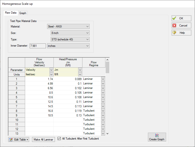
Entered Scaled Data: The data provided by Wilson, et al, 2006 for 203 mm (8 inch) pipe is as follows:
-
Material = Steel - ANSI
-
Size = 8 inch
-
Type = STD (schedule 40)
-
Raw Data table =
-
-
Table 1: Pressure drop data on phosphate slime from Wilson, et al, 2006 page 76 (203 mm/8 inch pipe)
| Parameters | Velocity | Jm | Flow Regime |
|---|---|---|---|
| Units | feet/sec | ft/ft | |
| 1 | 1.74 | 0.089 | Laminar |
| 2 | 4.99 | 0.100 | Laminar |
| 3 | 6.56 | 0.102 | Laminar |
| 4 | 8.50 | 0.105 | Laminar |
| 5 | 10.6 | 0.108 | Laminar |
| 6 | 12.5 | 0.110 | Laminar |
| 7 | 14.5 | 0.113 | Laminar |
| 8 | 16.8 | 0.119 | Turbulent |
| 9 | 18.5 | 0.130 | Turbulent |
-
In the table choose Velocity in
-
Click Create Graph at the bottom.
-
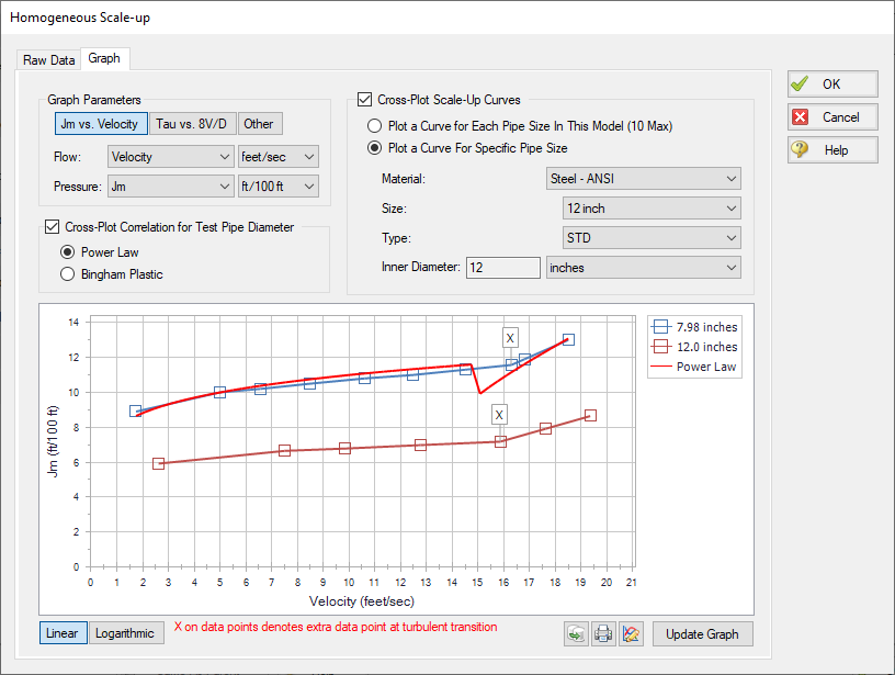
To see how the data will scale to 305 mm, choose the Cross-Plot Scale-Up Curves option, with Plot a Curve for Specific Pipe Size selected, specify the following parameters: Steel - ANSI, 12 inch, and STD
-
Click Update Graph at the bottom (see Figure 2)
-
To see how Power Law and Bingham Plastic model would work for this data choose them in the Cross-Plot Correlation for Test Pipe Diameter area.
-
Select OK
Step 3. Define the Pipes and Junctions Group
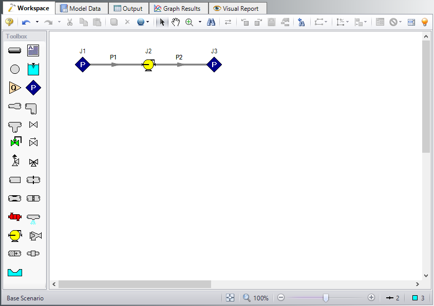
At this point, the first two groups are completed in Analysis Setup. The next undefined group is the Pipes and Junctions group. To define this group, the model needs to be assembled with all pipes and junctions fully defined. Click OK to save and exit Analysis Setup then assemble the model on the workspace as shown in the figure below.
Pipe Properties
-
Pipe Model tab
-
Pipe Material = Steel - ANSI
-
Pipe Geometry = Cylindrical Pipe
-
Size = 12 inch
-
Type = STD
-
Length =
-
| Pipe | Length |
|---|---|
| 1 | 1 inches |
| 2 | 2300 feet |
Junction Properties
-
J1 & J3 Assigned Pressure
-
Elevation = 0 feet
-
Pressure = 0 psig
-
Pressure Specification = Stagnation
-
-
J2 Pump
-
Pump Model tab
-
Name = 4755 gal/min
-
Inlet Elevation = 0 feet
-
Pump Model = Centrifugal (Rotodynamic)
-
Analysis Type = Sizing
-
Parameter = Volumetric Flow Rate
-
Fixed Flow Rate = 4755 gal/min
-
Nominal Efficiency = 75 Percent
-
-
Optional tab
-
Additional Efficiency Data
-
-
| Motor Power | Motor Eff. (%) |
|---|---|
| 100 | 95 |
-
Power Units = hp
Step 4. Create Two Alternate Cases
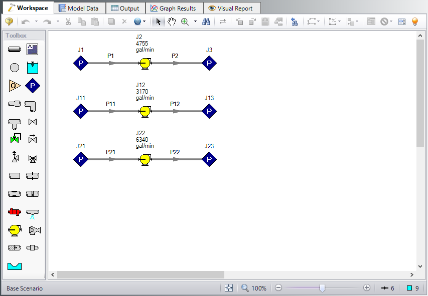
The example in Wilson et al, 2006, also requires evaluation of alternate flow rates. To create the alternate cases do the following:
-
Go to the Edit menu and click Select All
-
From the Edit menu again, select Duplicate Special
-
Increment All Pipe and Junction Numbers By = 10
-
Click OK
-
Move the duplicate below the first and click Paste
-
Repeat steps 2-5
-
For Pump J12, enter the following:
-
Name = 3170 gal/min
-
Fixed Flow Rate = 3170 gal/min
-
-
For the J22, enter the following:
-
Name = 6340 gal/min
-
Fixed Flow Rate = 6340 gal/min
-
The workspace should resemble Figure 4.
ØTurn on Show Object Status from the View menu to verify if all data is entered. If so, the Pipes and Junctions group in Analysis Setup will have a check mark. If not, the uncompleted pipes or junctions will have their number shown in red. If this happens, go back to the uncompleted pipes or junctions and enter the missing data.
Step 5. Run the Model
Click Run Model on the toolbar or from the Analysis menu. This will open the Solution Progress window. This window allows you to watch as the AFT Fathom solver converges on the answer. This model runs very quickly. Now view the results by clicking the Output button at the bottom of the Solution Progress window.
Step 6. Examine the Output
The Output window contains all the data that was specified in the Output Control window.
Figure 5 shows the Output window and includes the Pump Summary tab.
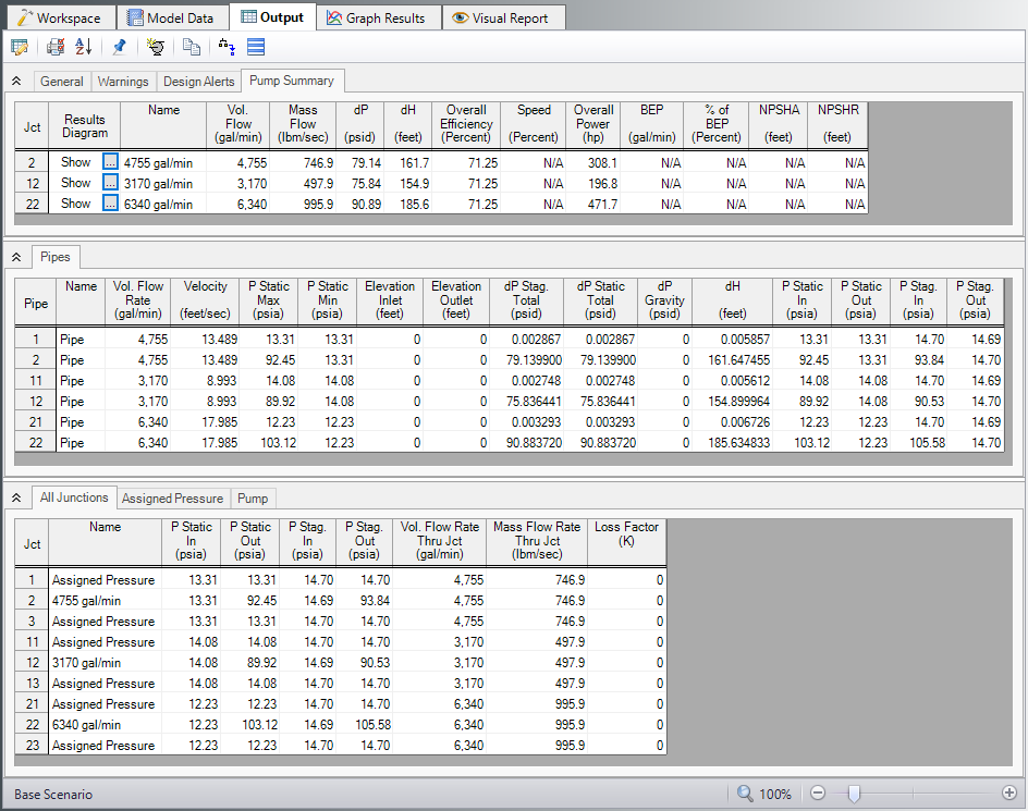
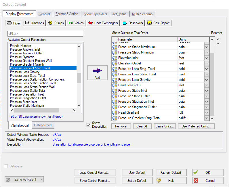
The Output Control window can be used to customize the output and to add output parameters.
-
Open Output Control from the toolbar or Tools menu
-
In the Pipes section choose Head Gradient and add it to shown output. Then change its units to
-
Next choose Pressure Gradient Stag. Total and add it. Then change its units to
-
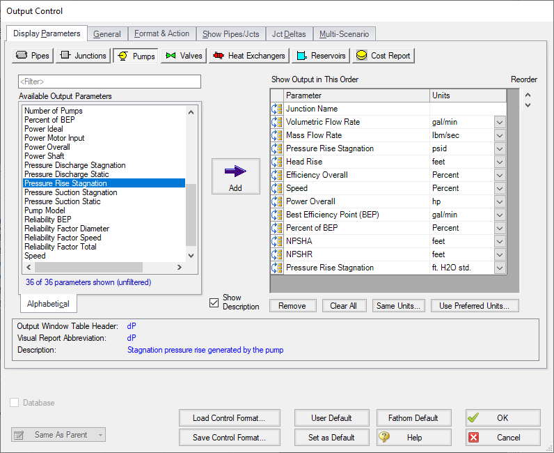
Select the Pumps button that runs along the top of Output Control.
-
Choose Pressure Rise Stagnation and add it. Then change its units to
-
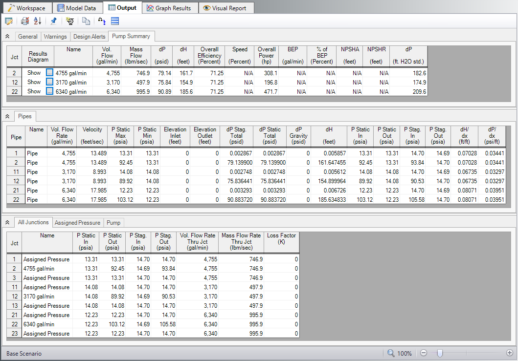
Click OK. The Output now appears as in Figure 8.
Table 3 summarizes the results from all three cases which agree well with those published by Wilson et al, 2006.
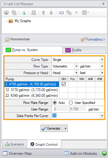
Also of interest is the system curve. Navigate to the Graph Results window by clicking the Graph Results tab on the toolbar, or by pressing Control+G. On the Graph Control tab in the Quick Access Panel, select the Pump vs. System Curve tab if not already selected. CRV for Pump 2 should be selected, see Figure 9. Click Generate.
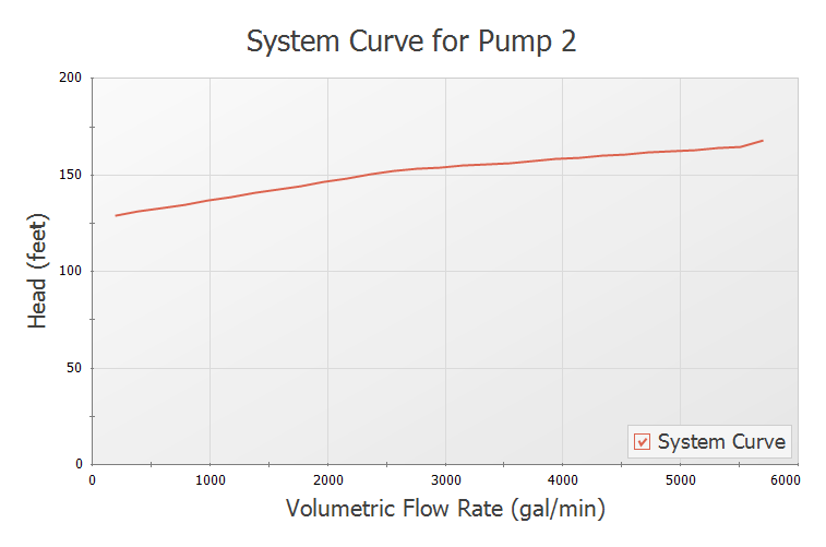
The system curve is shown in Figure 10.
Step 7. Compare Homogeneous Scale-Up to Power Law and Bingham Plastic Viscosity Models
Based on the fluid and flow regime and industry preference, a non-Newtonian model such as Power Law or Bingham Plastic may be preferred. How do those models compare to the Scale-up approach for the current example?
To perform the comparison, create two child scenarios. This can be done by opening the Scenario Manager on the Quick Access Panel. Create two child scenarios and call them Power Law and Bingham Plastic.
Here the Power Law scenario will be reviewed. The Bingham Plastic scenario will be very similar and hence is not shown. Results for all three scenarios will be compared later in this example.
-
Load the Power Law scenario
-
Open Analysis Setup
-
Open the Viscosity Model panel in the Fluid Properties group
-
Click the Enter Scaled Data button
-
Click the Graph tab
-
Select the Cross-Plot Correlation for Test Pipe Diameter option
-
Make sure the Power Law option is selected
-
If not, select it and click Update Graph
Figure 11 shows that the Power Law correlation matches the data well. The Bingham Plastic correlation diverges from test data at higher flow rates.
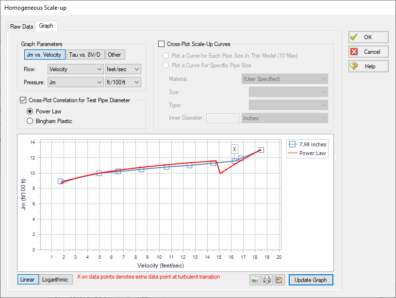
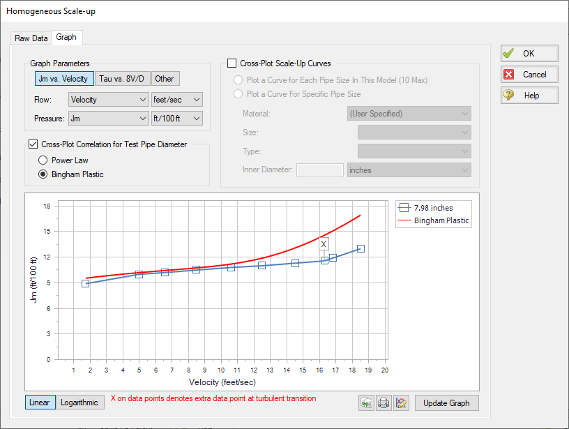
Figure 11: Non-Settling Slurry Scale-up data and Power Law (top) and Bingham Plastic (bottom) correlations
-
Click Cancel
-
Select Power Law from the drop down list of Viscosity Models
-
Select Calculate from Rheological Data
-
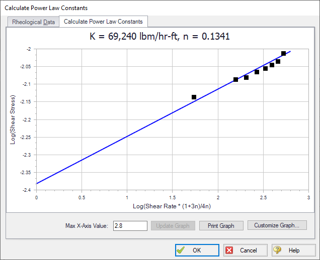
Click Calculate Constants
-
Make sure the Raw Data Type selection is Tube Flow Rheometer Data (8V/D)
-
Enter the shear rate and shear stress data from Table 2, below. This data is equivalent to the data from Table 1, entered previously. Alternatively, use theUS - Non-Newtonian Phosphates Pumping Rheological Data.txt file to import the shear rate and shear stress data into Fathom.
-
Click Generate Curve Fit Now
-
Click OK
The data should be K =
Table 2: Pressure drop data on phosphate slime from Wilson, et al, 2006 page 76 (203 mm/8 inch pipe) converted into shear rate (8V/D) and shear stress (Tau)
| Run | V | Jm | Shear Rate | Shear Stress |
|---|---|---|---|---|
| feet/sec | m/m | 1/seconds | psia | |
| 1 | 1.74 | 0.089 | 20.89 | 0.0073 |
| 2 | 4.99 | 0.100 | 59.90 | 0.0082 |
| 3 | 6.56 | 0.102 | 78.82 | 0.0083 |
| 4 | 8.50 | 0.105 | 102.1 | 0.0086 |
| 5 | 10.6 | 0.108 | 127.7 | 0.0088 |
| 6 | 12.5 | 0.110 | 150.2 | 0.0090 |
| 7 | 14.5 | 0.113 | 174.6 | 0.0092 |
| 8 | 16.8 | 0.119 | 201.8 | 0.0097 |
| 9 | 18.5 | 0.130 | 222.3 | 0.0106 |
Each scenario can be loaded and run. Results are summarized in Table 3. It is clear that the Bingham Plastic model over predicts the required pump head and power at higher flow rates but is comparable at the lowest flow rate of
Table 3: Comparison of results between Homogeneous Scale-up, Power Law, and Bingham Plastic models
| Q | gal/min | 3170 gal/min | 4755 gal/min | 6340 gal/min | ||||||
|---|---|---|---|---|---|---|---|---|---|---|
| Scale-Up | Power Law | Bingham Plastic | Scale-Up | Power Law | Bingham Plastic | Scale-Up | Power Law | Bingham Plastic | ||
| V | feet/sec | 8.993 | 8.993 | 8.993 | 13.489 | 13.489 | 13.489 | 17.985 | 17.985 | 17.985 |
| Jm | ft/ft | 0.06735 | 0.06846 | 0.06985 | 0.07028 | 0.07228 | 0.08079 | 0.08071 | 0.08210 | 0.10506 |
| dP/dx | psid/ft | 0.03297 | 0.03351 | 0.03420 | 0.03441 | 0.03539 | 0.03955 | 0.03951 | 0.04019 | 0.05144 |
| dP | psid | 75.84 | 77.09 | 78.66 | 79.14 | 81.39 | 90.97 | 90.89 | 92.45 | 118.31 |
| dH Water | feet | 174.9 | 177.8 | 181.4 | 182.6 | 187.7 | 209.8 | 209.6 | 213.2 | 272.9 |
| dH Fluid | feet | 154.9 | 157.5 | 160.7 | 161.7 | 166.3 | 185.8 | 185.6 | 188.8 | 241.7 |
| Power | hp | 196.8 | 200.0 | 204.1 | 308.1 | 316.8 | 354.1 | 471.7 | 479.8 | 614.0 |
Analysis Summary
A non-settling phosphate slurry pipeline was modeled and the pump sized for a range of flow rates. AFT Fathom non-settling slurry calculations allow evaluation of the non-Newtonian viscous behavior of the slurry.


