Plant Cooling Cost Calculation (English Units)
Summary
This example demonstrates the fundamental concepts of doing a cost analysis with AFT Fathom. The example illustrates how to calculate initial and life cycle costs for a given system design.
After designing a plant cooling system, it is necessary to calculate the system cost over a 10-year period to determine the feasibility of the design. The system model consists of four circulating water pumps, schedule 20 steel - ANSI pipes and fittings, and two sets of cooling tower cells.
To determine the cost of the cooling system for a 10-year period, include material, installation, and energy costs for the pumps, pipes, and fittings. The cooling towers costs will be determined apart from the system cost (cooling tower cost calculations are not included in this example).
Topics Covered
-
Creating cost libraries
-
Entering pipe, junction and fitting cost data into libraries
-
Connecting cost libraries
-
Using Cost Settings
-
Using the Cost Report
Required Knowledge
This example assumes the user has already worked through the Beginner: Three Reservoir Problem example, or has a level of knowledge consistent with that topic. You can also watch the AFT Fathom Quick Start Video Tutorial Series on the AFT website, as it covers the majority of the topics discussed in the Three-Reservoir Problem example.
In addition, it is assumed that the user has worked through the Controlled Heat Exchanger Temperature example and is familiar with the basics of doing cost calculations.
Model Files
This example uses the following files, which are installed in the Examples folder as part of the AFT Fathom installation:
-
Plant Cooling.dat - existing engineering library
-
Plant Cooling - Pump Costs.cst - completed cost library for Plant Cooling.dat
-
Plant Cooling - Elbow Costs.cst - completed cost library for AFT INTERNAL LIBRARY
-
Plant Cooling - Pipe Costs US.cst - completed cost library for Steel - ANSI
Note: The cost libraries above will be recreated as part of this example, but they are also included as reference material.
Step 1. Start AFT Fathom
From the Start Menu choose the AFT Fathom 12 folder and select AFT Fathom 12.
To ensure that your results are the same as those presented in this documentation, this example should be run using all default AFT Fathom settings, unless you are specifically instructed to do otherwise.
Step 2. Open the model
Open the US - Plant Cooling - Initial.fth model file listed above, which is located in the Examples folder in the AFT Fathom application folder. Save the file to a different folder.
The model should appear as shown in Figure 1.
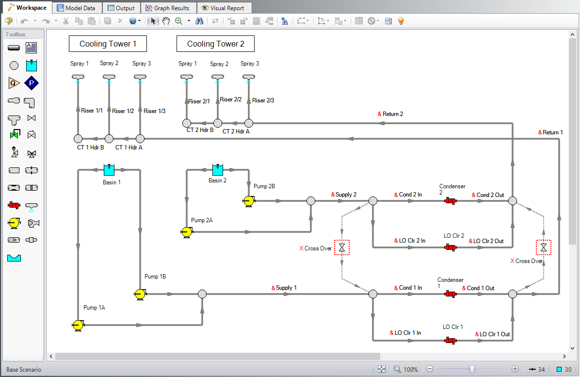
Figure 1: The Plant Cooling model (from the Examples folder in the AFT Fathom application directory)
Step 3. Define the Cost Settings group
By default, the cost calculations are turned off. To turn on the cost calculations, open Analysis Setup, navigate to the Cost Settings panel, and select Calculate in the Cost Calculation section. The Cost Settings panel is shown in Figure 2.
The Cost Definitions section allows you to specify the type of costs to be determined.
In the Cost Definitions area, select Material, Installation, and Operation/Energy costs by checking the box next to the name in the list.
In the Energy Cost section, select Use This Energy Cost Information, and enter a Cost of 0.06 U.S. Dollars Per kW-hr.
In the Cost Time Period section, enter a System Life of 10 years.
The Cost Settings panel should look like Figure 2. Close the Analysis Setup window by clicking OK.
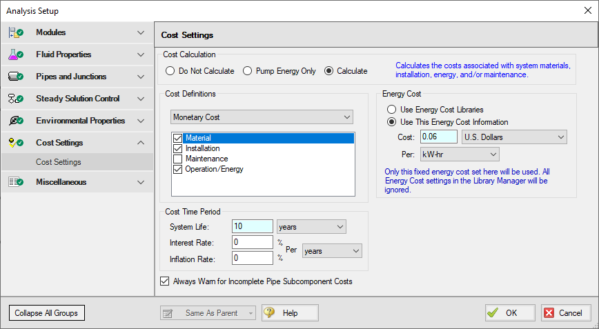
Figure 2: The cost calculations are selected on the Cost Settings window
Step 4. Create the Cost Libraries
Refer to the AFT Fathom Help Content for detailed information regarding creating and using cost libraries.
The energy cost for the pumps was specified in the Cost Settings as a fixed cost rate. Now, the material and installation cost for the pumps, pipes, and fittings must be included. This will be done by creating three new cost libraries.
The first cost library will be for the pipe material and installation costs and it will be associated with the engineering library that contains the pipe material data, which is the Steel - ANSI pipe material library.
The second cost library will be for the additional pipe fittings and losses costs for the elbow losses that are lumped into the pipes. The second cost library will be associated with the AFT INTERNAL LIBRARY. This is because the AFT Internal Library contains the loss information for the additional fittings and losses tab in the Pipe Properties window.
The third cost library will be for the pump material and installation costs, and it will be associated with the engineering library that contains the pump information (i.e., the Plant Cooling.dat engineering library).
Create a cost library for the pipe material and installation costs
Create a new cost library for the pipe costs by opening the Library menu and selecting Cost Library. Create a new cost library by clicking New at the bottom. When you click New, you are prompted to choose the engineering library with which the cost library will be associated.
The piping material data used in the model comes from the default Steel - ANSI Pipe Material Library, so the pipe cost library will be connected to this library, as well. Select Steel - ANSI from the library list shown in the Select Library window, then click Select.
Important: Make this choice carefully, because once you have made the association you cannot change it.
Once the library is created, you must enter a meaningful description and select the cost units. Enter the following data on the General tab:
-
Cost Type = Monetary
-
Monetary Unit = U.S. Dollars
-
Description = Plant Cooling - Pipe Costs
-
Notes = This library is for the Plant Cooling example File
Save the cost library to a file by clicking Save. Specify a file name such as, Plant Cooling - Pipe Costs US.cst, and click Save.
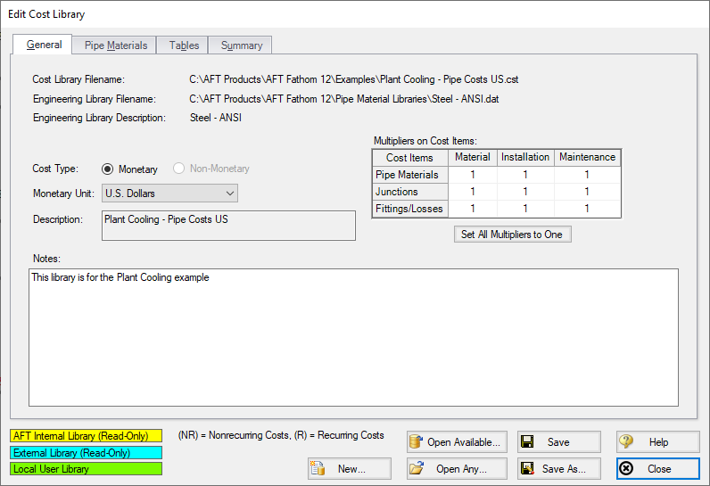
After saving, when prompted, choose to add the new library to the list of available and connected libraries by clicking Yes. The information on the General tab should appear as shown in Figure 3. The selected library file information, cost type and monetary units, a description of the cost library, and any descriptive notes you have added will be displayed.
Be sure to keep the Edit Cost Library window open for the next step. For this cost library, you will enter pipe material and installation costs on the Pipe Material tab.
Note: The library filenames may be different than those shown in Figure 3.
Enter the pipe material costs
After the pipe cost library has been created, select the Pipe Materials tab. This is where you will enter the material and installation costs for the piping.
The Pipe Materials tab shows all the pipes in the engineering library (AFT Steel - ANSI Pipe Material Library). Costs can be entered at several levels. You can enter costs at the material level, the nominal size level, and finally at the type (i.e., schedule) level. Costs entered at the material level apply to all nominal sizes and types in that material type. Costs entered at the nominal size level apply to all schedules within that nominal size. Costs entered at the type (schedule) level apply only to that type. For this example, all of the pipe material costs will be entered at the type (schedule) level for specific sizes.
To enter a new cost, start by switching the Sort selection to Material, Type or Schedule, Nominal Size. Navigate to Steel - ANSI, STD, 8 inch. Next click New Cost to create a new cost item in the table. The new cost item will appear as a new column.
Each pipe size in this example has two non-recurring (NR) costs associated with it. The costs to be entered are the material and installation costs. Figure 4 shows the costs entered for 8-inch STD Steel - ANSI. Enter the non-recurring pipe costs for the pipe in this example, as shown below.
All pipes are STD Steel - ANSI:
| Nominal Size (inches) | Material Cost (dollars/foot) | Installation Cost (dollars/foot) |
|---|---|---|
| 8 | 10.50 | 24.00 |
| 14 | 22.50 | 51.50 |
| 18 | 27.40 | 70.00 |
| 20 | 35.40 | 85.50 |
| 24 | 40.00 | 96.50 |
| 28 | 58.00 | 110.00 |
| 30 | 60.00 | 129.00 |
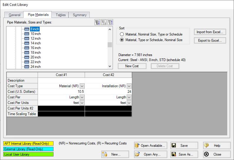
Figure 4: Non-recurring pipe costs, such as material and installation costs, are entered on the Pipe Materials tab
After the material and installation costs are entered for each STD type for the sizes listed above, click Save to save the information in the cost library file, and then click Close to close the Edit Cost Library window.
Create a cost library for the elbow fittings with cost scale tables
Several pipes in the model have 90 degree elbows specified in the Fittings and Losses tab in the respective Pipe Properties windows. The cost of these 90 degree elbow fittings can be included in the cost calculation. The costs for these items will be accounted for in scale tables. Scale tables can be used to vary a cost with a parameter such as diameter (i.e., size). Once created, this scale table can be applied to fittings and losses items.
Create a cost library for the elbow fittings and losses costs by opening the Library menu and selecting Cost Library. Create a new cost library by clicking New. You are prompted to choose the engineering library with which the cost library will be associated.
ØThe cost library for the elbow fittings and losses will be associated with the AFT INTERNAL LIBRARY, as this is the engineering library in which the pipe fittings and losses data is kept for the default elbow pipe fittings and losses. Select AFT INTERNAL LIBRARY and click Select.
On the General tab, specify the following information:
-
Cost Type = Monetary
-
Monetary Unit = U.S. Dollars
-
Description = Plant Cooling - Elbow Costs
-
Notes = This library is for the elbows included as additional Fittings and Losses for the pipes
Click Save and save this cost library with a file name such as Plant Cooling - Elbow Costs.cst
The first table to create is the scale table for the 90-deg. elbow installation costs. Select the Tables tab, and click New Table.
Enter the following data for the scale table on the New Scale Table window:
-
Name = 90 Elbows Installation
-
Table Type = Diameter
-
Table Format = Cost
After entering the data, click OK.
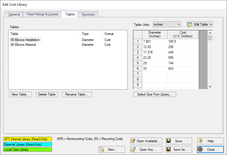
Now enter the cost data in the table using the values in the table below, as shown in Figure 5.
| Diameter (inches) | Installation Cost (US dollars) |
|---|---|
| 7.981 | 185.50 |
| 12.25 | 298.00 |
| 17.376 | 446.00 |
| 23.25 | 595.00 |
| 29.00 | 744.00 |
| 33.00 | 843.00 |
You do not need to enter data in the scale tables for every diameter in the model. If a diameter falls between two data points in the table, AFT Fathom will use the points on either side to linearly interpolate for a value. If the cost function is non-linear, you may need to add additional data points to achieve a more accurate cost value.
Create another scale table for the material costs using the following data:
-
Name = 90 Elbows Material
-
Table Type = Diameter
-
Table Format = Cost
| Diameter (inches) | Material Cost (US dollars) |
|---|---|
| 7.981 | 68.00 |
| 12.25 | 151.50 |
| 17.376 | 262.50 |
| 23.25 | 373.50 |
| 29.00 | 484.50 |
| 33.00 | 558.50 |
After the scale tables have been created, and the cost data entered, the Tables tab should appear as shown in Figure 5.
Click Save after the two cost tables are created and keep the Edit Cost Library window open for the next step.
Add the costs for pipe fittings
With the cost scale tables for the fittings defined, the costs for the pipe fittings can be added. Select the Pipe Fittings & Losses tab. A list of all of the available fittings and losses is displayed in the Pipe Fittings & Losses list.
The fittings in the model are Elbow/Bend, Smoothed Flanged, r/D=1, 90 deg. (C). Navigate through the list until you find the proper selection for these fittings.
Add the material cost by clicking New Cost, and entering the following data:
-
Description = Elbow Material Costs
-
Cost Type = Material (NR)
-
Material = Steel - ANSI
-
Material Size = All Sizes
-
Material Type = All Types
-
Use Size Table = Table of Costs
-
Multiplier = 1
-
Size Scaling Table = 90 Elbows Material
Now add the installation cost by clicking New Cost again and entering the following data:
-
Description = Elbow Installation Costs
-
Cost Type = Installation (NR)
-
Material = Steel - ANSI
-
Material Size = All Sizes
-
Material Type = All Types
-
Use Size Table = Table of Costs
-
Multiplier = 1
-
Size Scaling Table = 90 Elbows Installation
The actual cost values used for the fittings are the values that were entered in the scale tables on the Tables tab. The scale table to use for each cost is specified when the cost is defined. After the cost data is entered, the Pipe Fittings & Losses tab should appear as shown in Figure 6.
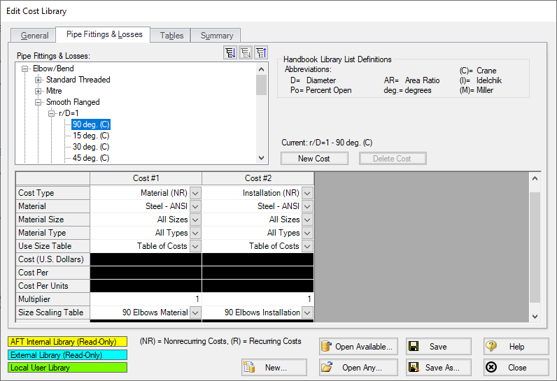
Figure 6: The Pipe Fittings & Losses tab in the Edit Cost Library window is used to specify costs for pipe fittings and losses items
Click Save and close the Edit Cost Library window, as now, the cost library for the elbow fittings and losses is now completed.
Create a cost library for the pumps
To enter cost for a pump, or any other junction type, the junction must first be added to the an engineering library in the Library Manager. Cost data is then entered in a cost library associated with that engineering library. The pumps used in this example have already been added to an engineering library, but no costs have been created for it yet. Create a new cost library associated with the Plant Cooling engineering library by opening the Library menu and selecting Cost Library.
Click New, then select the Plant Cooling library and click Select. Specify the following general information on the General tab:
-
Cost Type = Monetary
-
Monetary Unit = U.S. Dollars
-
Description = Plant Cooling - Pump Costs
-
Notes = This library is for the pumps in the Plant Cooling engineering library
Save the cost library to a file by clicking Save and giving the file a name such as Plant Cooling - Pump Costs.cst. When prompted, choose to add the new library to the list of available and connected libraries. Keep the Edit Cost Library window open for the next step.
Enter the pump costs
After the pump cost library has been created, select the Junctions tab. This is where you will enter the material and installation costs for the pumps.
All of the junctions that are available in the selected engineering library will be listed. Select the
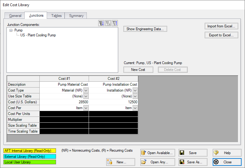
Add the material cost by clicking New Cost, and entering the following data:
-
Description = Pump Material Cost
-
Cost Type = Material (NR)
-
Use Size Table = (None)
-
Cost (U.S. Dollars) = 28500
-
Cost Per = Item
Add the installation cost by clicking New Cost again and entering the following data:
-
Description = Pump Installation Cost
-
Cost Type = Installation (NR)
-
Use Size Table = (None)
-
Cost (U.S. Dollars) = 12500
-
Cost Per = Item
Figure 7 shows the pump costs entered in the cost library.
Click Save and then click Close.
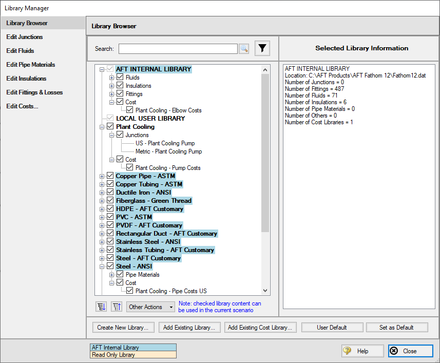
Connecting the cost libraries
The Plant Cooling engineering and cost libraries should have been added to the list of available libraries and been connected to the example model. If they were not, you can use the Library Manager to connect the cost libraries now (see Figure 9). The Plant Cooling - Pump Costs is connected subordinate to the Plant Cooling. The Plant Cooling - Pipe Costs
Make sure that the pumps are utilizing the engineering library junction data, otherwise the costs will not be calculated.
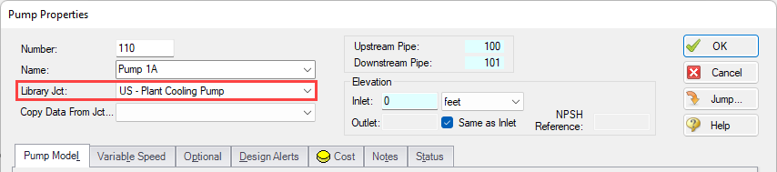
Figure 8: Pump using the engineering library data
Step 5. Including objects in the Cost Report
The final step before performing a cost analysis is to specify which pipes and junctions you want to be included in the final cost report. This is done by opening the properties window, navigating to the Cost tab, and choosing Include in Cost Report for each pipe and junction to be included, as shown for Pipe 100 in Figure 10.
Include the four circulating water pumps and all of the pipes in the cost report. The Global Edit feature may be used to update this information for all of the pumps and pipes.
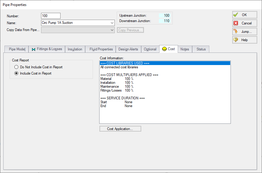
Figure 10: The Cost tab on the Pipe and Junction Properties windows is used to include the objects in the Cost Report
Step 6. Run the Model
Click Run Model on the toolbar or from the Analysis menu. This will open the Solution Progress window. This window allows you to watch as the AFT Fathom solver converges on the answer. This model runs very quickly. Now view the results by clicking the Output button at the bottom of the Solution Progress window.
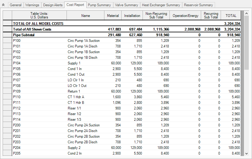
Step 7. Examine the Cost Report
The Cost Report is displayed in the General Results section of the Output window. View the Cost report by selecting the Cost Report tab. The content of the Cost Report can be modified from the Output Control window. Figure 11 shows the Cost Report for this example with the Material, Installation, Operation/Energy, and Total costs displayed.
The Cost Report shows the total system cost, as well as the individual totals for the material, installation, and energy costs. In addition, the Cost Report displays the detailed cost for each pipe, junction, and fitting that was included in the report. The items are grouped together by type, and a subtotal for each category is listed.
Analysis Summary
The cost analysis for this example shows the following costs for the plant cooling system design:
| Total of All Model Costs | $3,204,334 |
| Total Material Cost | $417,883 |
| Total Installation Cost | $697,484 |
| Total Operation/Energy Cost | $2,088,968 |
| Total Cost of Pipe | $918,940 |
| Total Cost of Pumps | $2,252,968 |
| Total Cost of Fittings | $32,426 |
Minimizing Cost with AFT Fathom Automated Network Sizing Module™
The AFT Fathom Automated Network Sizing Module (ANS) is a tool built on AFT Fathom technology. With the ANS module you can automatically size all pipes or ducts in your system to minimize monetary cost, weight, volume, or surface area. In addition, you can concurrently size the pumps and pipes to obtain the absolute lowest cost system that satisfies your design requirements. Finally, by accounting for non-recurring and recurring costs, you can size pipe and duct systems to minimize life cycle costs over some specified duration.
By using the AFT Fathom Automated Network Sizing Module (ANS) on this example, not only could the system cost be determined, the cost could also be minimized by varying selected pipe and junction sizes in the system.


