Beginner: Filling a Tank - XTS (English Units)
Beginner: Filling a Tank - XTS (Metric Units)
Summary
The objective of this example is to introduce the user to the Extended Time Simulation (XTS) module by modeling the filling of a tank. A liquid transfer system will be modeled. The pump will run for a specified time, and the change in fluid height in the delivery tank will be examined using the transient output data.
Note: This example can only be run if you have a license for the XTS module.
Topics Covered
-
Specifying Transient Control
-
Understanding Transient Output
Required Knowledge
This example assumes the user has already worked through the Walk-Through Examples section, and has a level of knowledge consistent with the topics covered there. If this is not the case, please review the Walk-Through Examples, beginning with the Beginner: Three Reservoir Model example. You can also watch the AFT Fathom Quick Start Video Tutorial Series on the AFT website, as it covers the majority of the topics discussed in the Three-Reservoir Model example.
Model File
This example uses the following file, which is installed in the Examples folder as part of the AFT Fathom installation:
Step 1. Start AFT Fathom
From the Start Menu choose the AFT Fathom 12 folder and select AFT Fathom 12.
To ensure that your results are the same as those presented in this documentation, this example should be run using all default AFT Fathom settings, unless you are specifically instructed to do otherwise.
Step 2. Define the Modules Panel
Open Analysis Setup from the toolbar or from the Analysis menu. Navigate to the Modules panel. For this example, check the box next to Activate XTS and select Transient to enable the XTS module for use. A new group will appear in Analysis Setup titled Transient Control. Click OK to save the changes and exit Analysis Setup. Open the Analysis menu to see the new option called Time Simulation. From here you can quickly toggle between Steady Only mode (normal AFT Fathom) and Transient (XTS mode).
Step 3. Define the Fluid Properties Group
-
Open Analysis Setup from the toolbar or from the Analysis menu.
-
Open the Fluid panel then define the fluid:
-
Fluid Library = AFT Standard
-
Fluid = Water (liquid)
-
After selecting, click Add to Model
-
-
Temperature = 70 deg. F
-
Step 4. Define the Pipes and Junctions Group
At this point, the first two groups are completed in Analysis Setup. The next undefined group is the Pipes and Junctions group. To define this group, the model needs to be assembled with all pipes and junctions fully defined. Click OK to save and exit Analysis Setup then assemble the model on the workspace as shown in the figure below.
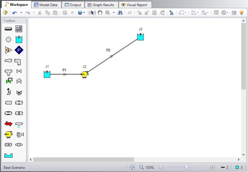
The system is in place but now we need to enter the properties of the objects. Double-click each pipe and junction and enter the following properties. The required information is highlighted in blue.
Pipe Properties
-
Pipe Model tab
-
Pipe Material = Steel - ANSI
-
Pipe Geometry = Cylindrical Pipe
-
Size = 4 inch
-
Type = STD (schedule 40)
-
Friction Model Data Set = Standard
-
Lengths =
-
| Pipe | Length (feet) |
|---|---|
| 1 | 10 |
| 2 | 990 |
Junction Properties
-
J1 Reservoir
-
Name = Lower Reservoir
-
Tank Model = Infinite Reservoir
-
Liquid Surface Elevation = 10 feet
-
Liquid Surface Pressure = 0 psig
-
Pipe Elevation = 0 feet
-
-
J2 Pump
-
Inlet Elevation = 0 feet
-
Pump Model = Centrifugal (Rotodynamic)
-
Analysis Type = Pump Curve
-
Enter Curve Data =
-
| Volumetric | Head |
|---|---|
| gal/min | feet |
| 0 | 300 |
| 500 | 380 |
| 1000 | 250 |
-
Curve Fit Order = 2
-
J3 Reservoir
-
Name = Upper Reservoir
-
Tank Model = Finite Open Tank
-
Known Parameters Initially = Liquid Surface Level & Surface Pressure
-
Cross-Sectional Area = Constant, 150 feet2
-
Liquid Level Specification = Height from Bottom
-
Liquid Height = 0 feet
-
Liquid Surface Pressure = 0 psig
-
Tank Height = 30 feet
-
Pipe Elevation = 200 feet
-
Tank Bottom Elevation = 200 feet
-
Step 5. Define the Transient Control Group
XTS module transient simulations are controlled through the Transient Control group in Analysis Setup. Access the Transient Control group by opening the Simulation Duration panel. When Fathom is set to perform a transient analysis, Transient Control becomes one of the items required to run the model.
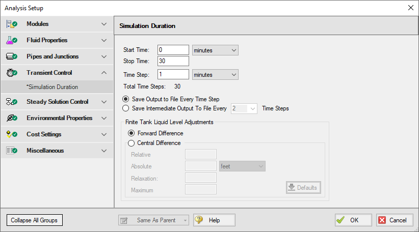
The Simulation Duration panel in the Transient Control group is used to specify transient start and stop times, as well as the time step controls and solution parameters for finite tank liquid level calculations. Start times, stop times, and time steps can be specified in any units from seconds to years. From the Simulation Duration panel, users can specify the number of output points that are saved to the transient output file. This allows XTS to do transient calculations with a small time step while limiting the size of the transient data output file. Enter the following inputs in the Simulation Duration panel, as shown in Figure 2.
-
Start Time = 0 minutes
-
Stop Time = 30
-
Time Step = 1 minutes
In addition to Transient Control, it is possible in define transient events for individual junctions. This allows the user to define events such as pump trips or start-ups, or valve closures. For this example, we will not specify any junction transients. The transient data for this example will be related to the fluid being pumped into the tank over the transient time period we have defined in Transient Control.
Step 6. Specify the Time Simulation Formatting
Open the Output Control window and select the Format & Action tab. Set the Time Simulation Formatting units to minutes and click OK to save and close the window.
ØTurn on Show Object Status from the View menu to verify if all data is entered. If so, the Pipes and Junctions group in Analysis Setup will have a check mark. If not, the uncompleted pipes or junctions will have their number shown in red. If this happens, go back to the uncompleted pipes or junctions and enter the missing data.
After all of the pipes and junctions have been defined, and all of the transient data and transient control items have been specified, the transient simulation may be executed.
Step 7. Run the Model
Click Run Model on the toolbar or from the Analysis menu. This will open the Solution Progress window. This window allows you to watch as the AFT Fathom solver converges on the answer. This model runs very quickly. Now view the results by clicking the Output button at the bottom of the Solution Progress window.
When using the XTS module, the Solution Progress window displays the progress through the transient analysis. This information is displayed below the solution tolerance data, as shown in Figure 3:
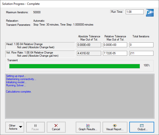
Figure 3: Solution Progress Window shows the convergence progress, as well as the transient solution progress when running transient cases
Step 8. Examine the Output
AFT Fathom displays transient output for all Pipes and Junctions in the Output Window, as shown in Figure 4.
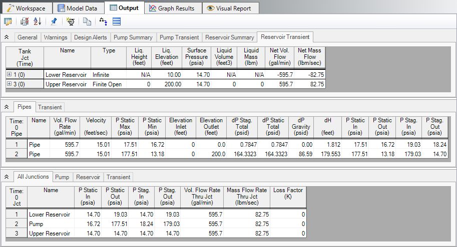
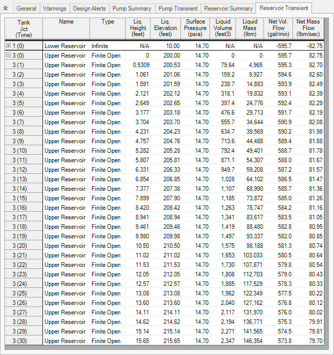
Each of the summary tables in the General Output section has a companion transient summary tab which displays the summary data at each time step in the transient run. Each junction included in the summary is included in the transient summary. The transient summary data for each junction may be expanded or collapsed by clicking the + or – sign in beside the junction data list. The entire list may be expanded or collapsed by clicking the button in the top left-hand corner of the transient summary window. Figure 5 shows the Reservoir Transient summary tab, with all of the data sets collapsed. Figure 6 shows the Reservoir Transient summary tab, with the data for the J3 Reservoir expanded.
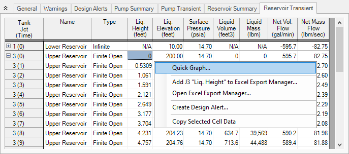
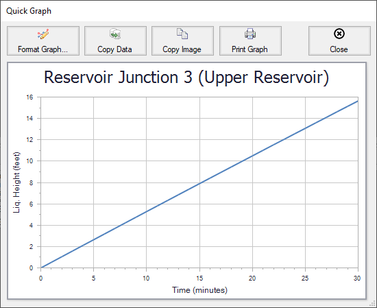
The Quick Graph feature can be used to quickly plot transient data for quick examination. To use the Quick Graph feature, place the mouse cursor over the column of data you wish to examine. Then, right click with the mouse, and select Quick Graph from the list. Figure 7 illustrates how to do this for J3 Reservoir Liquid Height vs. Time. Figure 8 shows the resulting graph. The graph illustrates how the liquid level in the Reservoir rises with time, as would be expected. The Graph Results window may also be used to create a full range of graphs related to the XTS module transient output.
Similar to the summary transient data, the transient tabs in the Pipe and Junctions sections of the Output Window are used to display the transient data for each pipe and junction at every time step, as shown in Figure 9. This transient data can be expanded or collapsed in the same manner as in the General Output transient summaries.
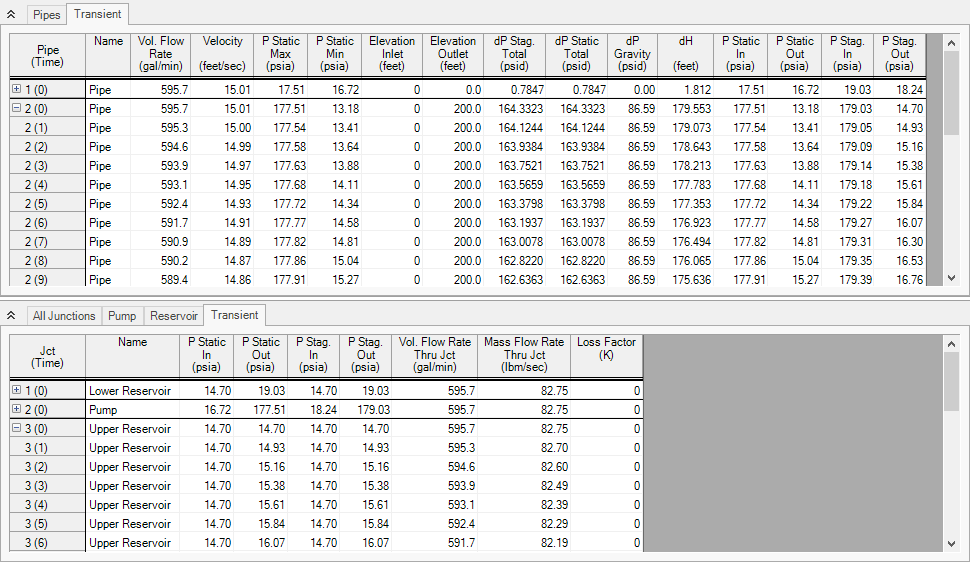
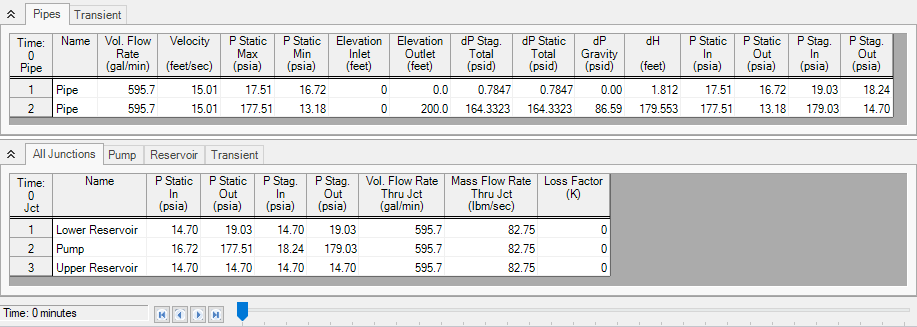
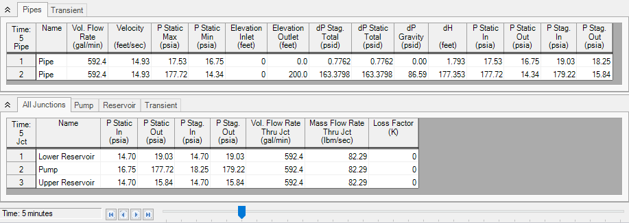
Figure 10 shows the output data for the pipes and junctions, found on the Pipes and All Junctions tabs, at the initial time step, Time = 0 minutes. The output for all of the pipes and junctions can be displayed at any time step by using the slider bar located at the bottom of the Output window. Figure 11 shows the pipe and junction data at Time = 5 minutes.
Step 9. Create a New Scenario
Create a new scenario called Variable Speed Pump.
Open the Pump Properties window for J2. On the Variable Speed tab, set the pump to Controlled Pump (Variable Speed) and select Volumetric Flow Rate with a Control Setpoint of
Rerun the model.
Step 10. Examine the Output
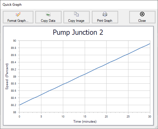
Figure 12 shows a Quick Graph plot of the Pump Speed vs. Time for the controlled flow pump. Note how the pump speed increases over time to maintain the controlled flow. This is because the hydrostatic pressure downstream of the pump is increasing because the tank is slowly filling over time.