Improved ATKF Method
For commercial steel pipe and pipes with a similar roughness, it has been shown that the equivalent length, Darby 3-K, and Adjusted Turbulent K Factor (ATKF) methods will all produce similar results in the laminar flow region (see Adjusted Turbulent K Factor (ATKF) Method).
However, this is not the case when the pipe roughness varies significantly from that of commercial steel. At different roughness values the predicted head loss with the original ATKF method varies inversely with pipe roughness, so that smoother pipes will experience higher head loss in the laminar regime as is shown in Figure 1. The Darby 3-K method shows no dependence on pipe roughness in the laminar regime, as is shown in Figure 2. It would be expected that head loss in the laminar regime would behave as predicted by the 3-K method, based on the fact that the laminar friction factor is independent of pipe roughness.
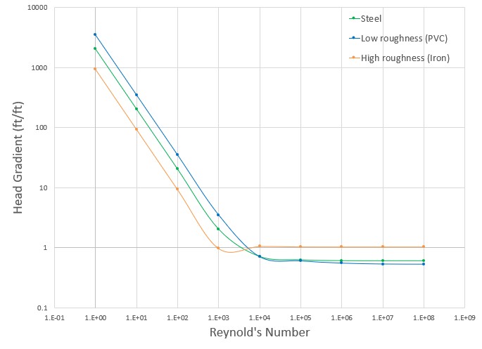
Figure 1: Head Gradient calculated with the original ATKF method at different roughness values, showing differences in the laminar region
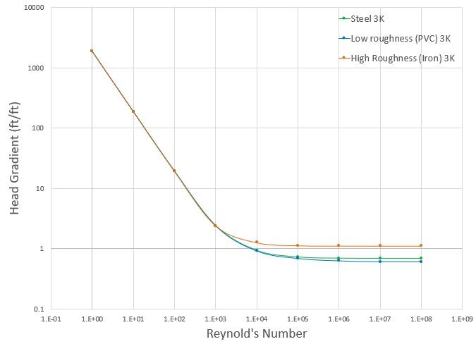
Figure 2: Head Gradient calculated with the 3-K method at different roughness values, showing no differences in the laminar region
To remove the dependence on pipe roughness in the ATKF method, the Improved ATKF method uses a fixed turbulent friction factor value calculated for commercial steel pipe (roughness 0.0018 in) at very large Reynolds numbers. The Improved ATKF method can be written as follows, replacing fturb with the reference turbulent friction factor, fturb,ref :

With the Improved ATKF factor it can be seen that the head loss is no longer dependent on pipe roughness (Figure 3).
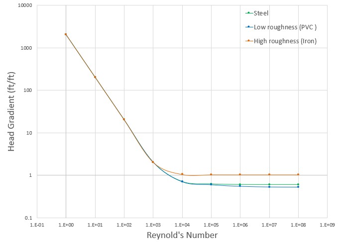
Figure 3: Head gradient calculated with the Improved ATKF method at different roughness values
Related Topics
Laminar and Non-Newtonian Corrections Panel
Adjusted Turbulent K Factor Method (ATKF)
Related Blogs
Applying the Improved ATKF Method for Laminar and Non-Newtonian Flow


