Adjusted Turbulent K Factor Method (ATKF)
Crane (1988)Crane Co., Flow of Fluids Through Valves, Fittings, and Pipe, Technical Paper No. 410, Crane Co., Joliet, IL, 1988. includes an equivalence between equivalent length methods and K-factor on the nomograph chart on page A-30. This nomograph is based on theory as discussed below.
The basic law of pressure drop for friction factor is
|
|
(1) |

For K-factors the pressure drop is given by
|
|
(2) |

From equations 1 and 2 it can be seen that there is an equivalence between f*L/D and K.
The equivalent length method works by adding to the physical length as follows:
|
|
(3) |

Hence the pressure drop due to the methods can be related as follows:
|
|
(4) |

An appropriate equivalent length can be determined from standard AFT Fathom K-factor data by looking at large Reynolds number and hence fully turbulent conditions
|
|
(5) |

And finally a general K-factor which is based on equivalent length can be found in the following:
|
|
(6) |

To apply the method, take the AFT Fathom K-factors (Kturb) and multiply them by the relevant pipe friction factor, f, at actual conditions (and Reynolds number) and divide them by the turbulent friction factor, fturb, evaluated at very large Reynolds number.
Improved ATKF Method
For the Improved ATKF method, the turbulent friction factor in equation 6 is is replaced with the turbulent friction factor calculated for commercial steel at very large Reynolds numbers,which is about 0.023 for a roughness of 0.0018 in. This allows the adjusted K factor to be independent of pipe roughness in the laminar flow region so that it more closely mimics the expected behavior for the 3K method from DarbyDarby, R., Chemical Engineering Fluid Mechanics, 2nd edition, Marcel Dekker, New York, NY, 2001. and the equivalent length method.
Comparison of Equation 6 to Published Data
A study was performed to evaluate how Equation 6 compares to published data (Wood 2012D. Wood, T.W Walters, "Operational problems in pumping non-settling slurries resolved using an improved laminar pipe fitting loss model" in 28th Intern. Pump Users Symp., Houston Texas, Turbomachinery Laboratory, Texas A&M University, 2012). A comparison for a 10 foot long, 2 inch in diameter pipe flowing water was performed with the following:
-
No fittings in the pipe
-
Fittings of 12 elbows of 1.5 r/D with a total K of 3.17 but no corrections (this is the way standard AFT Fathom works)
-
Darby 3-K method for 12 elbows
-
Equivalent length of 12 elbows with Leq/D = 16 (see Darby, 2001, pp.209)
-
Use Equivalent Length in Pipe Diameters (L/D) Derived From K-Factors, Eq. 6
Figure 1 shows the results on a log-log plot. One would not expect the first case to match the others as no fittings were included. Hence the head gradient was less than the other cases. However, Case 1 does illustrate how Case 2 works in the standard AFT Fathom. Case 2 agrees with Cases 3-5 at high Reynolds Number but agrees with Case 1 at low Reynolds number. This is a result of using turbulent, high Reynolds Number K-factors for low Reynolds Number applications.
Cases 3, 4 and 5 all agree well throughout the entire range of Reynolds Numbers. There is some small discrepancy at high Reynolds Number which is merely a result of various reference differences over the exact pressure loss through a 1.5 r/D elbow.
The conclusion from Figure 1 is that the Equation 6 method allows reliable adjustment of turbulent pressure loss data for fittings and junctions to laminar applications.
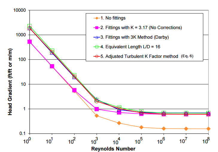
Figure 1: Log-log plot of dimensionless head gradient vs. Reynolds number for various fitting loss models
Related Topics
Laminar and Non-Newtonian Corrections Panel
Related Blogs
Applying the Improved ATKF Method for Laminar and Non-Newtonian Flow


