Role of Pressure Junctions - Detailed Discussion
In modeling a generalized pipe network, it is possible to construct models that do not have a unique solution. A common occurrence of this is when a model contains one or more sections which are completely bounded by known flow rates. A series of examples with accompanying explanation will clarify situations where this occurs.
Before beginning, it will be helpful to consider an aspect of the philosophy of computer modeling. At the risk of stating the obvious, it must be recognized by the user that a computer model cannot calculate anything that cannot in principle be calculated by hand. All the computer does is accelerate the calculation process. Some users expect the model to generate independent information and become frustrated when the software requests additional information from them. But if the user was doing the calculation by hand that same information would still be required. The difference is that in the case of the hand calculation, the engineer would be forced to think through why the information is needed.
However, when the engineer interacts with AFT Fathom, they do not need to think at the same depth as in the hand calculation. So when AFT Fathom asks for the additional information, it is not as apparent why it is required. This disconnect in thinking can cause frustration for the user. Fully understanding the concepts in this topic will greatly reduce the frustration for some users, and will improve the quality of models for all users.
Examples
The simplest example is the system shown in Figure 1. In AFT Fathom terms, the system has two assigned flow junctions. Heat transfer has no affect on the point being made here and is therefore ignored in all examples.
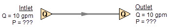
Figure 1: Model with two assigned flows. This model does not have a unique solution.
Obviously, the flow in the pipe is known. But what is the pressure at the inlet? At the outlet? It cannot be determined because there is no reference pressure. The reference pressure is that pressure from which other pressures in the system are derived. There can be one or more reference pressures, but there always has to be at least one.
The model in Figure 1 can be built with AFT Fathom and if you try and run this model, AFT Fathom will inform you that it cannot run it because of the lack of a reference pressure. In AFT Fathom there are several junctions that can act as a reference pressure: the reservoir, assigned pressure, spray discharge, valve (with the exit valve option), orifice (with the exit orifice option), and exit type relief valves when open.
There are a couple other things worth noting about Figure 1. First is that the model in Figure 1 has redundant boundary conditions. When one flow is specified in a single pipe, the other end must have the same flow. Thus the second known flow does not offer any new information. Because the conditions are redundant, there is no unique solution to the model in Figure 1. In any AFT Fathom model, there is always at least one unknown for each junction in the model – either pressure or flow rate. Sometimes there are two unknowns, such as a Pump. It is possible the user may not know either the flow or the pressure at the pump. In such cases the user is required to specify the relationship between flow and pressure. This relationship is called a pump curve, and by specifying the relationship between the two, effectively one of the two unknowns can be eliminated. Thus we always end up with one unknown for each junction.
Second, if the user was allowed to specify two flows as in Figure 1, they could specify them with different flow rates. Both ends of the pipe must have the same flow, so an inconsistency occurs. The basic reason the inconsistency is possible is because Figure 1 does not have a unique solution.
Figure 2 a-c shows three alternate configurations for the model in Figure 1. It is not possible to specify inconsistent conditions for any of the Figure 2 models, and they always have a unique solution no matter what input is specified by the user.
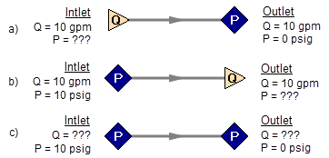
Figure 2a-c: Top two models with one pressure and one assigned flow, bottom model with two pressures. All of these models have a unique solution.
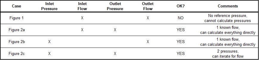
The four models in Figures 1 and 2 a-c contain all logical possibilities. In all four cases there are four things we want to know. The pressure and flow at the inlet, and the pressure and flow in the outlet. In each case we know two of these four. The problem is that in the Figure 1 model the lack of a reference pressure makes it impossible to determine the inlet and outlet pressures, even though we know the flow. The three models in Figure 2 a-c all have at least one pressure and thus all four of the desired parameters can be determined. Table 1 summarizes this. Also note in Table 1 that in the Figure 2c case the flow can be determined, but it is by iteration.
Table 1: Four logical possibilities of boundary conditions for single pipe systems
As we consider multi-pipe systems, there are a host of other possibilities that present themselves. All other configuration possibilities which lack a reference pressure ultimately boil down to the same problem that exists in Figure 1.
The pipe lengths, diameters and friction factors are not included in the remaining models because they do not influence the main point of this topic. It is assumed that these parameters can be obtained for each pipe and the resulting pressure drop calculated with standard relationships.
Consider the model in Figure 3. With three boundaries having a known flow, this clearly has the same problem as the model in Figure 1. No unique pressures at any location can be calculated.
A pressure at any one of the three boundaries in Figure 3 would be sufficient to allow a unique solution of the system. It is also possible that there could be two pressures and one flow, or three pressures. As long as there is at least one pressure a unique solution exists.
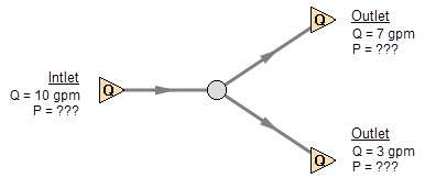
Figure 3: Three known flows at boundaries lack a reference pressure, similar to the model in Figure 1. This model does not have a unique solution.
Now consider the models in Figure 4. The Figure 4a model does have one reference pressure, but in this case there is still a problem. The Flow Control Valve (FCV) is controlling the flow to 10 gpm, and the downstream flow is demanding 10 gpm. The section of the system before the FCV can be solved (because there is a pressure upstream), but the section after the FCV does not have a unique solution. Why? In order to obtain a unique solution, the pressure drop across the FCV must be known. But any pressure drop could exist and satisfy the conditions of this model. It is thus not possible to determine the pressure at the outlet flow demand because it depends on the FCV pressure drop which is not known. The model in 4b does have a pressure downstream of the FCV, and thus there is a unique pressure drop across the FCV and a unique solution exists for the model in Figure 4b.
If you input the remaining data for the Figure 4a model and run it in AFT Fathom, you will get the message shown in Figure 5. AFT Fathom identifies the part(s) of the model where a known pressure is needed.
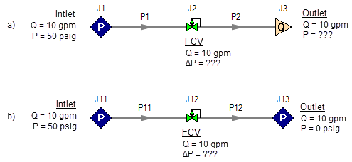
Figure 4a-b: The model at the top does not have a reference pressure after the Flow Control Valve so the pressure drop across the FCV cannot be determined. The top model does not have a unique solution. The bottom model has a pressure upstream and downstream, and a unique solution exists
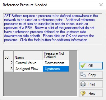
Figure 5: AFT Fathom message when you try to run the model shown in Figure 4a
Sizing Pumps with Flow Control Valves
An analogous situation to Figure 4a is when the user is trying to size a pump using the Pump with a fixed flow. The Pump with a fixed flow is really just a reverse FCV. It controls the flow by adding pressure, rather than reducing it. Figure 6 shows this case and is another example of a model without a unique solution, requiring more than one pressure junction. If the user instead entered a pump curve for this model, it could be solved.
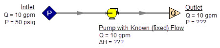
Figure 6: A pump modeled as a fixed flow behaves identically to the FCV model in Figure 4a, for which no unique solution exists
Increasing in model complexity, Figure 7 shows some additional examples of models without a unique solution. In particular, Figure 7b has a pump with a fixed flow that can add as much pressure as it wants, and the downstream FCV can then take out as much as it wants. There are an infinite number of possible solutions.
While it would be highly unusual for a system to have two FCV’s in series, it is worth considering the model in Figure 7b further. It is common to have an FCV in series with a pump. How does one size the pump in such a case? There are several ways to do this, one of which is to change the pump from a fixed flow to an actual pump curve. Trying multiple pump curves will guide you to the best pump.
But there is a better way. Consider for a moment the pressure drop across the FCV in Figure 7b. In the installed system, is any pressure drop acceptable? Usually not. It is typical to have pressure drop limits based on the system design and the FCV itself. A common requirement is a minimum pressure drop across the FCV. If no minimum pressure drop exists, let’s say we choose a pump that results in the pressure drop across the FCV being 0.01 psid. If the system is built and the pump slightly underperforms its published curve, the FCV will not be able to control to its flow control point. Even if the pump does operate exactly on the published curve, eventually fouling in the pipes will result in increased pipe resistance (and pressure drop) and again the FCV will not be able to control to its flow control point.
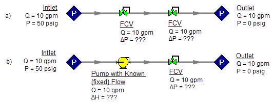
Figure 7: Neither model above has a unique solution. The top model has two flow control valves in series. The bottom model has a pump modeled as a fixed flow in series with an FCV. In both cases either a third pressure junction is needed between the two middle junctions, or one of the junctions must be changed from a flow controlling device.
To avoid these kinds of problems in installed systems, a minimum Cv or pressure drop across the FCV is typically required. This minimum pressure drop provides the key to sizing the pump in Figure 7b. Rather than model the FCV as a flow control valve, instead model it as a pressure drop control valve (PDCV) set to the minimum pressure drop requirement. Then a unique solution exists, the model will run and the pump can be sized. Once the pump is sized and an actual pump curve exists, the pump curve can be entered for the pump and the valve can be switched back to an FCV. Remember that when we use the PDCV, we are still getting the flow we want for the true FCV, because the pump is now providing the control.
Think for a moment what we just did. We went through a thought process that many engineers have gone through during their hand calculations. Specifically, we size the pump such that the FCV pressure drop is minimized. If the FCV has a larger pressure drop than the minimum, the pump must pump harder to overcome this excess pressure drop. In short, it must use more energy and is thus less efficient. Figure 8 depicts this process.
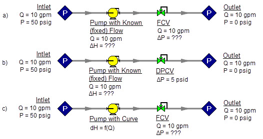
Figure 8a-c: The model at the top is the same as Figure 7b and does not have a unique solution. To size the pump, change the model to the second one shown above, which uses a pressure drop control valve (PDCV) rather than an FCV. Once the second model is run, the pump is sized, a pump curve exists, and the model at the bottom can be run using an FCV.
Let’s make a slight addition in complexity to the model in Figure 8. In this case we have two flow control valves in parallel (Figure 9). To size this pump, we apply the process described in Figure 8. We choose one of the FCV’s, make it a PDCV, size the pump, choose a pump with an actual pump curve and enter it into the model, then return the PDCV to an FCV.
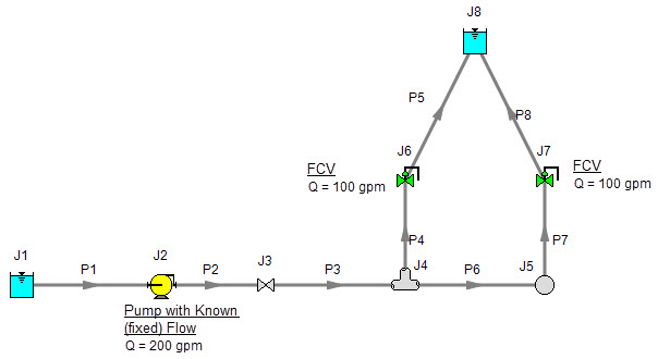
Figure 9: A pump with a fixed flow in series with two parallel FCV’s. The model in its current form does not have a unique solution. To size the pump, first change the FCV at J7 to a PDCV.
This brings up the question, which FCV should one choose to turn into a PDCV? When FCV’s are put in parallel, frequently the pipe design has one of the FCV’s further away from the pump than the others. Because of the additional piping leading to this FCV, it will be the weakest link in the chain of parallel FCV’s by virtue of having the lowest pressure drop across it. The most remote FCV should be chosen as the PDCV. If the most remote FCV is chosen, when the minimum pressure drop required is applied to the PDCV all other FCV’s in the parallel system will have greater than the minimum pressure drop — thus satisfying the pressure drop requirement for those FCV’s as well.
What if you do not know which FCV is the most remote? In this case make your best guess, change it to a PDCV at the minimum required pressure drop, run the model, then verify whether all other FCV’s have a pressure drop that meets or exceeds the requirement. If not, then the FCV with the smallest pressure drop as determined by the first run is in reality the weakest FCV. Choose this FCV, change it to a PDCV, and then change the original PDCV back to an FCV since it is not the weak link. If the pipe system leading to each FCV is truly identical and all FCV’s have identical pressure drops, any of the FCV’s will serve as the PDCV.
The preceding process can be extended to cases where there are three or more FCV’s in parallel, and also cases with more than one pump in parallel supplying the FCV’s.
In Figure 9 the most remote valve is J7, the one on the right. If the minimum pressure drop is 5 psid, change J7 to a PDCV with a 5 psi drop. This results in the output shown in Figure 10a. Notice how the pressure drop across the other FCV at J6 (6.837 psid) is greater than 5 psid because it is closer to the pump. Also notice how the flow through J7 is still 100 gpm even though it is not controlling flow. Once again, the reason for this is that the pump is controlling the flow to 200 gpm, and with the J6 FCV controlling to 100 gpm, the excess must go through J7. The pump is thus sized and its pump pressure rise is shown in Figure 10b (127 ft.).
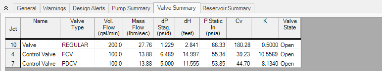
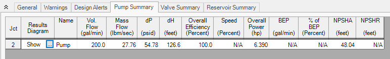
Figure 10a-b: Results from changing J7 in Figure 9 to pressure drop control valve
Using Fixed Head Rise Pumps
An alternate method of sizing pumps with FCV’s is to use the fixed head rise pump model. Here the pump head can be adjusted while the flow control valves can be modeled as FCV’s. This approach is particularly powerful when used with theGSC Module. This would entail specifying the pump head rise as the variable at the min Cv or pressure drop across the control valve as the goal. If there are multiple, parallel control valves, then a group max/min can be used.
Pressure Control Valves
The problem of non-unique solutions can also occur when a Pressure Reducing Valve (PRV) or Pressure Sustaining Valve (PSV) is used. A PRV is used to control pressure downstream of the valve, while a PSV controls pressure at the valve inlet. One thing that PRV’s and PSV’s have in common with FCV’s is that the pressure drop cannot be known ahead of time. The pressure drop depends on the balance of the pipe system.
Consider the simple system shown in Figure 11. With the pressure controlled downstream of the PRV, the pressure upstream is not known. Without knowledge of the PRV’s pressure drop, the pressure upstream of the PRV cannot be determined and thus no unique solution exists.
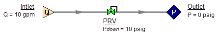
Figure 11: If a PRV is downstream of a known flow the PRV pressure drop cannot be calculated. This model does not have a unique solution.
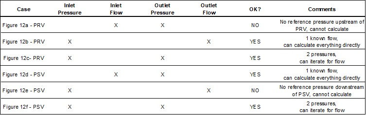
Figure 12 shows the possible cases with PRVs and PSVs, while Table 2 comments on the six cases. In summary, at least one known pressure is always needed on the side of a pressure control valve opposite of the controlled side.
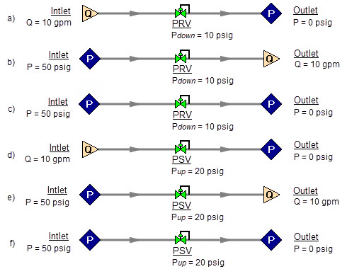
Figure 12a-f: Six possibilities for PRV and PSV configurations. Cases A and E do not have unique solutions. See Table 2 for comments.
Table 2: Summary of six possibilities for PRV and PSV configurations.
If a pump is being sized in series with a PRV or PSV, modeling the pump as a fixed flow will not permit a unique solution if the pump is upstream of a PRV or downstream of a PSV. The reasons for this are the same as those in the previous section on FCV’s.
In combination with the previous examples, it should be apparent how the non-unique solution problem can occur in more complicated systems. In all such cases, the reasoning will boil down to the same problems already discussed.
Closing Parts of a System
A model may be built which has sufficient information to obtain a unique solution. Then a user closes a pipe or junction and all of a sudden the problem of no unique solution occurs. This is shown in Figure 13. The top model has a unique solution and will run fine. In the bottom model the valve is turned off and the section of the system downstream of the valve has only known flows. No reference pressure exists in this section because it is isolated from the known pressures in the section on the left.
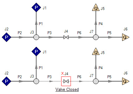
Figure 13: Top model has reference pressures at J1 and J2. Bottom model has closed valve at J4 which isolates the J5 and J6 assigned flows. There is no reference pressure for J5 and J6 and no unique solution exists for the bottom model.
Summary
AFT Fathom models always require one reference pressure, and may require more if the engineer uses control valves, pumps with fixed flows, or closed pipes or junctions. The actual number of reference pressures needed depends on the model, but AFT Fathom always checks to be sure sufficient reference pressures exist and stops to warn the user when they do not.
This capability is a powerful diagnostic feature that will help guide the user in building meaningful models.
Related Blogs
Reference Pressure Needed: Where It Comes from and How to Address it


