Role of Pressure Junctions and How They Work
In modeling a generalized pipe network, it is possible to construct models that do not have a unique solution. A common occurrence of this is when a model contains one or more sections which are completely bounded by known flow rates.
The simplest example is the system shown in Figure 1. In AFT Fathom terms, the system has two assigned flow junctions.
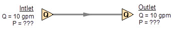
Figure 1: Model with two assigned flows. This model does not have a unique solution.
Obviously, the flow in the pipe is known. But what is the pressure at the inlet? At the outlet? It cannot be determined because there is no reference pressure. The reference pressure is that pressure from which other pressures in the system are derived. There can be more than one reference pressure, but there always has to be at least one.
The model in Figure 1 can be built with AFT Fathom and if you try and run this model, AFT Fathom will inform you that it cannot run it because of the lack of a reference pressure (Figure 2). In AFT Fathom there are several junctions that can act as a reference pressure: the reservoir, assigned pressure, valve (with the exit valve option), orifice (with the exit orifice option), spray discharge, relief valve junctions which are open to an external pressure, and pressure control valves.
When you try and run a model that has one or more sections completely bounded by known flows (or Flow Control Valves or Pumps operating in fixed flow mode), the Need Reference Pressure window (shown below) is displayed. This window informs you which junctions bound the sections where a reference pressure is needed to obtain a unique solution.
In multi-pipe systems there are a host of other possibilities that present themselves. All other configuration possibilities which lack a reference pressure ultimately boil down to the same problem that exists in Figure 1.
See Role of Pressure Junctions - Detailed Discussion for more information.
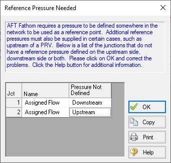
Figure 2: AFT Fathom message when you try to run a model without sufficient reference pressures
How Pressure Junctions Work
Pressure junctions (e.g., reservoirs or assigned pressures) in AFT Fathom are an infinite source or sink of fluid. This means that they can draw or discharge as much fluid as is necessary to maintain the specified pressure. This section offers a physical example of how pressure junctions work.
Consider the physical pumping system shown in Figure 3. This system pumps water from Lake Ontario to Lake Huron.
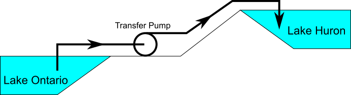
Figure 3: Physical pumping system to transfer water from shoreline supply tank (J1) to discharge tank (J2) at top of hill
An engineer is tasked with sizing the pump for this system. The engineer has an idea of the discharge head needed for the pump, and so builds an AFT Fathom model as shown in Figure 4. The Figure 4 model is attempting to represent the physical system in Figure 3, but it in fact represents the physical system in Figure 5.
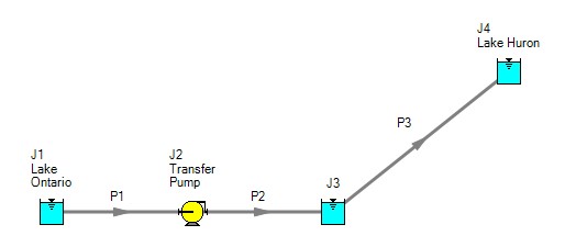
Figure 4: Model to size pump attempting to represent system in Figure 3. It does not accurately represent Figure 3
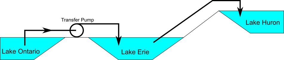
Figure 5: Physical system represented by model in Figure 4
Why? Because the reservoir junction (J3), which is an infinite source of fluid, has been located between the pump (J2) and Lake Huron (J4). The J3 reservoir isolates Lake Ontario and the pump (J1 and J2) from Lake Huron (J4). The J3 reservoir is very much like placing Lake Erie between the supply and discharge piping.
If the engineer changes the surface elevation in J3, it is like changing the surface elevation of Lake Erie. It will change the flow rate in the pipes, but no matter how high the water level of Lake Erie, it does not change the fact that the pumping system is isolated from Lake Huron. The flow rate in the piping from J4 to J3 is entirely dependent on the difference in surface elevations between J3 and J4, and is not influenced by the J2 pump in any way.
How then should the physical system in Figure 3 be modeled? It should be modeled as shown in Figure 6.
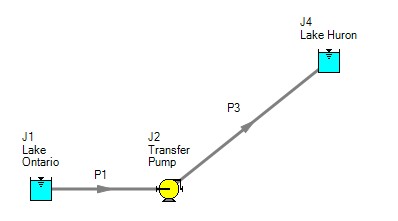
Figure 6: Proper model of physical system shown in Figure 3
If the goal is to size the pump at J2, the model in Figure 6 can be used with the pump modeled as a fixed flow pump.
Related Topics
Role of Pressure Junctions - Detailed Discussion
Convention for Positive Flow Direction
Features for Modeling Irrecoverable Losses
Philosophy of Computer Modeling
Stagnation vs. Static Pressure Boundaries
Related Examples
Related Blogs
Reference Pressure Needed: Where It Comes from and How to Address it


