Slurry Definition Panel
(SSL Module Only) The Slurry Definition panel allows selection of the Slurry Model and related options such as the Slurry Calculation Method, as well as input of solids concentration relative to the carrier fluid and estimation of bulk slurry properties, as shown in Figure 1.
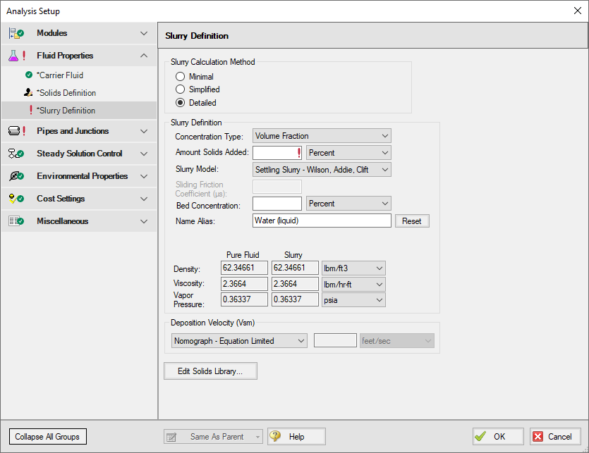
Figure 1: Slurry Definition panel when Detailed Slurry Calculation Method and User Specified Solids Added are selected
Slurry Calculation Method
There are three calculation methods available to model slurries when using the Wilson, Addie, Clift slurry model. These are all variations of the Wilson, Addie, Clift slurry approach, and this selection is only applicable when Settling Slurry - Wilson, Addie, Clift is chosen as the active Slurry Model in the Slurry Definition panel. Each method requires different amounts of input data resulting in the use of different calculations. These calculations are described in the Slurry Calculation Methods section.
-
Minimal Method - Used in the preliminary design phase where only rough data are available. The solids density, sliding friction coefficient, and solids concentration are the only parameters needed. However, due to the minimal data the calculations should only be used for early stage approximations because it often over-predicts losses. This is a conservative method that assumes a fully-stratified sliding bed.
-
Simplified Method - Additional information is required and gives a better solution. This method requires the solids density, d50 particle size, a user-specified M exponent, and the solids concentration. This method assumes heterogeneous flow with suspended particles. This is a more accurate model than the Minimal method because it accounts for more slurry definition.
-
Detailed Method - The default and provides the most rigorous solution methodology. The solids density, d50 particle size, terminal velocity parameter, and the solids concentration are required. Additionally, if the M exponent is to be calculated, the d85 particle size is also required. As with the Simplified Method, this method also assumes heterogeneous flow with suspended particles.
The Concentration Type is used to specify a value in the Amount Solids Added field. The available options for Concentration Type are:
-
Grams per Liter of Mixture
-
Volume Fraction
-
Mass Fraction
-
Solids Ratio (M-solids/M-liquid)
There are a few Slurry Model options to choose from. These options determine the calculations used in the Solver.
-
Newtonian - Functionally disables most of the SSL module calculations and preserves only the viscosity properties of the fluid in the model.
Note: The No Solids Added option from the Solids Definition panel is only compatible with the Newtonian Slurry Model option. If you have already specified solids on the Solids Definition panel, you must select one of the other Slurry Models below.
-
Settling Slurry - Wilson, Addie, Clift - Default option, applies slurry calculations from the Wilson, Addie, Clift Slurry Models.
-
Settling Slurry - 4-Component Model - The 4-Component Slurry Model developed by GIW Industries Inc. - A more complex model that takes into consideration the contribution of different size particles in the slurry flow.
-
Wasp-Durand Heterogeneous Model - The Wasp-Durand Slurry Model is a two-layer slurry approach with heterogeneous and homogenous fluid components.
The Sliding Friction Coefficient (μs) is the coefficient of mechanical sliding friction between the granular mass and the boundary - where the boundary is where the motion takes place between the mass and a rigid boundary, i.e. the pipe wall. As the Sliding Friction Coefficient increases, so does the friction and thereby the pressure drop through the pipe. Typical values range from 0.4 to 0.5. This field is only available when the Wilson, Addie, Clift Minimal Slurry Calculation Method or the 4-Component slurry model are selected.
The Bed Concentration (Cvb) is an optional parameter for the Wilson, Addie, Clift slurry methods and is only used to determine the actual settling velocity (Vs) shown in the output. These calculations are described in Wilson (1986)Wilson, K.C., “Effect of Solids Concentration on Deposit Velocity”, Journal of Pipelines, 5, 1986, pp. 251-257. and are functions of the pipe diameter, particle size (d50), particle density and relative concentration. If no value is entered for this parameter then a default of 0.60 is used. The maximum value of these settling velocities (Vs) is denoted Vsm and is the usual parameter of interest in designing a system to avoid operating with a stationary bed. This field is only available when the Simplified and Detailed Slurry Calculation Methods are specified at the top of the panel.
The Deposition Velocity (Vsm) can be determined using one of the options below. This is useful when the calculation method yields a slightly different value than, say, test results.
-
Nomograph - Equation Limited (Wilson, Addie, Clift only) - This option is the default and uses the nomograph from Wilson (1986)Wilson, K.C., “Effect of Solids Concentration on Deposit Velocity”, Journal of Pipelines, 5, 1986, pp. 251-257. page 111. The nomograph is noted to be conservatively high by Wilson, so an equation that calculates the max Vsm is used to limit the value of Vsm.
The results calculated from the nomograph will be checked against Equation 5.11 from Wilson (1986) as is shown below. If the value from the nomograph exceeds Vsm,max calculated from Equation 5.11, then the Vsm,max from Equation 5.11 will be used instead.

Note: If the Vsm is calculated as a negative value using Equation 5.11 from Wilson then the Vsm will be displayed as 0 in the Output. If the Vsm is shown as 0, the inputs for the fluid and solid should be verified, and the user should consider calculating the Vsm using a separate method.
-
Equation Only (Wilson, Addie, Clift only) - This option will cause the Vsm to be calculated solely using Equation 5.11.
-
User Specified (Wilson, Addie, Clift only) - This option allows the user to directly specify Vsm.
-
Note: As Wilson describes there are times where operating at a velocity lower than Vsm is economically attractive and is without a stationary bed. These cases include a system where the solid concentration at the desired operating point is very different than that at the Vsm conditions. Wilson points out that this is rarely the case, and so the use of Vs instead of Vsm should be done with caution.
-
Nomograph Only (4-Component only) - This option will cause deposition velocities to be calculated from the Wilson, Addie, Clift nomograph, similar to the Nomograph - Equation Limited Wilson, Addie, Clift option without the limiting equation. The other notable difference is that two deposition velocities are calculated for the 4-Component method from two different diameters; Vsm,h from d50h and Vsm,s from ds.
-
Match Heterogeneous Calculation (Wasp-Durand only) - The calculation method for Wasp-Durand deposition velocities is coupled to the selection of the Heterogeneous Gradient Calculation Method. The following methods are used, which are described in more detail in Wasp-Durand Heterogeneous Slurry Model:
-
Wasp-Durand
-
Liu Dezhong
-
Fei Xiangjun
-
When using the Wasp-Durand Slurry model, the Wasp-Durand Options section will be displayed within the Slurry Definition panel. Equations associated with these options may be found in the Wasp-Durand Heterogeneous Slurry Model section.
The Sedimentation Velocity Model determines which model is used to calculate sedimentation velocity, which is calculated per particle size group and is a particle settling velocity. This is the terminal particle freefall velocity that occurs when the drag, gravity, and buoyancy forces on a particle are balanced. There are two options available. Either option is appropriate for a wide range of flow states and particle sizes, including laminar, transitional, and turbulent flow, so the selection of model will depend on personal preference or industry standards:
The Heterogeneous Gradient Calculation Method determines the set of equations to use for calculating the heterogeneous component of the slurry pressure gradient, along with the deposition velocity, as these options are always coupled for Wasp-Durand. Three options are available:
The Apply Apparent Slurry Properties option allows the viscosity of the homogeneous (vehicle) component to be affected by solids, or specified by the user manually. Without this option enabled, the clear fluid carrier fluid viscosity will be used. The following viscosity options are available when applying apparent slurry properties:
-
User Specified Viscosity - The viscosity used for the homogeneous pressure gradient is specified by the user rather than being inherited from the carrier fluid or calculated from the carrier fluid and particle size distribution. This option treats the homogeneous component as Newtonian.
-
Apply Viscosity Model - These options calculate the carrier fluid viscosity including the contribution of solids. Solids of all sizes will contribute to the homogenous viscosity, but finer particles contribute more significantly.
-
Thomas (1965) - This can be used to calculate a Newtonian viscosity value or Bingham stiffness factor for each pipe.
-
Fei Xiangjun - Mineral - This method calculates a Newtonian viscosity or Bingham stiffness factor for each pipe, and can also calculate a global yield stress value for the slurry.
-
Fei Xiangjun - Coal - This method is mathematically identical to the Fei Xiangjun - Mineral viscosity models, but the empirical values are tuned to coal slurry data rather than mineral slurries.
-
When active, the Use Hanks' Bingham Plastic Friction Model checkbox replaces the Newtonian homogeneous component friction calculations with a non-Newtonian Bingham plastic approximation. With this option, yield stress may be manually specified or calculated using the Fei Xiangjun methods. The Bingham stiffness factor is calculated iteratively for each pipe using the Fei Xiangjun or Thomas (1965) methods.


