Check Valve
The Check Valve junction type requires two connecting pipes. This junction type allows you to model the effect of a check valve which closes to prevent back flow.
The Check Valve Properties window follows the first of the two basic Properties window formats, displaying the connecting pipes in a fixed format. The Check Valve junction does not have an explicit flow direction, but adopts a flow direction from the connecting pipes for calculating loss. The user can define the base area for the loss model, though the default is set to use the upstream flow area.
A check valve is a device that allows flow in only one direction. AFT Impulse assumes that the Check Valve is initially open (unless modeled as Closed on the Optional tab). If the flow solution indicates that the system hydraulics are insufficient to keep the check valve open based upon the check valve input, AFT Impulse closes the valve. The valve can close during the steady-state or transient portion of the simulation.
AFT Impulse allows you to model the check valve by entering a User Specified closing velocity, using valve performance data to Estimate from Fluid Deceleration, or with a Force Balance calculation. Further details about each of these types of check valve are discussed below.
For all of these options the Loss Model for the open valve can be specified as a Cv, Kv or K factor by choosing an option on the Valve Model tab and entering the Full Open value.
User Specified
The User Specified option opens and closes based on user-defined values for velocity to close and a delta pressure to reopen. For steady-state analysis the valve is either fully open, or fully closed. In a transient analysis, the valve opens and closes instantaneously.
The inputs are as follow:
-
Forward Velocity to Close Valve - By default this value is zero. Some valves are designed to start closing at some reverse velocity - you can specify that here as a negative value. Entering a positive value in this field would imply that the check valve closes while the flow is still continuing forward.
-
Delta Pressure/Head to Reopen - Frequently after a check valve closes, there is pressure across the valve at which it will open again. You can specify that delta pressure here.
Estimate from Fluid Deceleration (no reopen)
This option attempts to predict the maximum reverse velocity at which the valve will close. This maximum velocity is based on experimental predictions involving fluid deceleration and various check valve types from Thorley, 2004 Thorley, A.R.D., Fluid Transients in Pipeline Systems, 2nd Ed., D&L George, Ltd. 2004 (pages 241-243). Once the fluid deceleration is determined, the chart for Maximum Reverse Velocity vs. Fluid Deceleration is used to determine the Forward Velocity to Close for the check valve. If the deceleration is above the range given in the chart for the specific valve type selected, the transient run will be terminated, and a different valve type must be selected. Once the check valve closes, it will not reopen.
There are three options provided to choose the Valve Performance Data Type that will be used for the Maximum Reverse Velocity vs. Fluid Deceleration chart.
-
Non-dimensional - The non-dimensional data sets are provided from Thorley, 2004 Thorley, A.R.D., Fluid Transients in Pipeline Systems, 2nd Ed., D&L George, Ltd. 2004 and Ballun, 2007 Ballun, John V., "A Methodology for Predicting Check Valve Slam", Journal AWWA, Vol.99, No. 3, pp. 60-65, March 2007. . If this option is chosen, the user must provide the Minimum Velocity Required to Fully Open Valve, which is then used to find the Dimensionless Maximum Reverse Velocity.
-
Dimensional - This option uses the original dimensional data from Thorley, 2004 Thorley, A.R.D., Fluid Transients in Pipeline Systems, 2nd Ed., D&L George, Ltd. 2004 and Ballun, 2007 Ballun, John V., "A Methodology for Predicting Check Valve Slam", Journal AWWA, Vol.99, No. 3, pp. 60-65, March 2007. , eliminating the need to convert to dimensionless values. This option may not be appropriate if the valves being modelled are not similar to the valve sizes used to obtain the experimental data. The dimensional data from Thorley was obtained using several sizes: the Moving Ball and Swing types used DN 100 (approximately 4 inches), the Split Disc types used DN 200 (approximately 8 inches), and the Nozzle types used DN 300 (approximately 12 inches). The Ballun data used a size of DN 200 (approximately 8 inches).
-
User Defined - If dimensional data is available for the Maximum Reverse Velocity vs. Fluid Deceleration from the manufacturer, this option allows the user to directly define the curve to be used.
The Deceleration Calculation Interval is an optional input which allows the user to specify the time interval used to calculate the fluid deceleration. See the Deceleration Calculation Interval section below for further explanation. The resultant deceleration values can be viewed in the Output window.
Force Balance
Force Balance data can be used to model two valve types, Swing Check and Translating Nozzle/Plug valves. Both models are based on work published in Wylie, et al, 1993Wylie, E.B., V.L. Streeter & L. Suo, Fluid Transients in Systems, Prentice Hall, Englewood Hills, New Jersey, 1993..
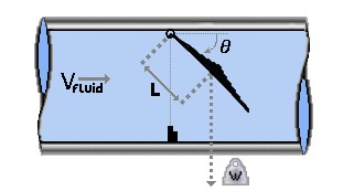
Figure 1: Swing Check valve diagram
The Swing Check Valve model uses a torque balance to estimate rate and position over time for a swing check valve. The inputs for the swing check valve are as follows (reference Figure 1):
-
Disk Properties
-
Distance to CG (L) - The distance from the pivot point to the disk assembly center of gravity.
-
Area (A) – The surface area of the disk.
-
Weight (submerged, W) - The submerged weight of the disk assembly. If you do not know this value for the check valve you are trying to model, refer to the Approximating Submerged Weight for the Swing Check Valve section.
-
Inertia (I) - The moment of inertia of the disk about the pivot point. If you do not know this value for the check valve you are trying to model, refer to the Approximating Disk Inertia for the Swing Check Valve section.
-
Mass of Displaced Fluid - By default, a mass of fluid equal to the mass of a sphere of fluid the same diameter as the valve disk is added to the valve inertia term. The user can specify a custom fluid mass to be included by choosing User Specified, or choose to neglect the fluid mass entirely by choosing None.
-
Valve Loss vs. θ Data - The fully open (minimum) angle and the fully closed (maximum) angle of the disk must be defined, as shown in the diagram. Additionally the Cv vs. θ data must be defined in the table. A warning will be given to the user if the data in the table is inconsistent with the specified fully open and fully closed angles, or with the specified fully open Cv.
-
Include Spring
-
Spring Constant (k) - The torsional spring stiffness, if a spring is present. The value is zero if there is no spring.
-
Spring Torque With Valve Closed (T) - The residual torque exerted by the spring when valve is fully closed. The value is zero if there is no spring torque when the valve is closed.
-
Custom Orientation - By default, the orientation will be assumed to be horizontal which is shown in parentheses when the box is unchecked. Enabling this box allows the user to either specify the valve orientation as vertical, or for a user specified angle as measured from horizontal.
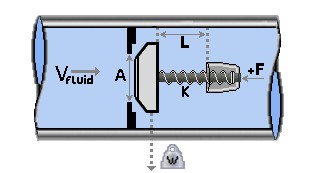
Figure 2: Translating nozzle/plug check valve diagram
The translating disk/plug check valve inertia model is solved using the force balance equation, the valve equation, and the positive and negative characteristic equations. The inputs are as follows (reference Figure 2):
-
Nozzle/Plug Properties
-
Max Travel Length (L) - The distance the disk/plug travels from fully closed to fully open.
-
Area (A) - The cross-sectional surface area of the disk/plug perpendicular to the flow.
-
Weight (W) - The weight of the disk/plug assembly.
-
Mass of Displaced Fluid - By default, the displaced fluid mass will be calculated using the distance travelled by the nozzle/plug. The user can specify a custom fluid mass to be included by choosing User Specified, or choose to neglect the fluid mass entirely by choosing None.
-
Valve Loss vs. Travel Length - Variation of valve Cv in terms of Travel Length to Fully Open.
-
Spring Properties
-
Spring Constant (k) - The linear spring stiffness, if a spring is present. The value is zero if there is no spring.
-
Spring Force with Valve Closed (F) - The residual force exerted by the spring when valve is fully closed. The value is zero if there is no spring force when the valve is closed. This is used to calculate Xs, the spring length at which the spring force is zero.
-
Custom Orientation - By default the orientation will be assumed to be horizontal, which is shown in parentheses when the box is unchecked. Enabling this box allows the user to either specify the valve orientation as vertical, or for a user specified angle as measured from horizontal.
Deceleration Calculation Interval
This optional input is only applicable when using the Estimate from Fluid Deceleration check valve model. AFT Impulse needs to use the fluid deceleration to calculate the velocity at which the check valve will close (and therefore the time step of closure). Due to certain transient behavior in a model, the deceleration may vary over time. For example, see Figure 3 below where the slope of the blue line changes over time. However, the Valve Performance Data (either the aforementioned Thorley/Ballun data or a user defined curve) will need a single deceleration value to calculate the fluid velocity at closure (Max Reverse Velocity). Therefore, Impulse will approximate the deceleration using the slope of a linear line from the time of initial deceleration (point 1) to the time when reverse velocity starts (point 2), as seen in the black dashed line. The default deceleration calculation might not accurately predict the velocity at which the check valve closes due to the slope of the blue and black lines differing at point 2.
The Deceleration Calculation Interval allows the user to manually specify a value for the time interval over which the slope (deceleration) is calculated. This effectively moves point 1 to a different time step. Impulse will then use the slope of the red dashed line as the value for deceleration. In this case shown in Figure 3, the default method likely provides a more conservative estimate because higher deceleration (steeper slope) would result in a larger Max Reverse Velocity, which then can result in a larger hydraulic force from check valve slam.
Note: This option is best used after you have already run the model, analyzed a Velocity vs Time graph, and determined that the deceleration (slope of the Velocity curve) differs significantly over time. In some cases using this setting may produce a less conservative estimate for a pressure/force spike (ex. pump trips), while other times it will produce a more conservative estimate (ex. valve closure elsewhere in the system where the effective closure time is short).

Figure 3: Example plot demonstrating how Impulse approximates the fluid deceleration for the Estimate From Fluid Deceleration Check Valve Model
Approximating Disk Inertia for the Swing Check Valve
The swing check valve model requires the user to input the disk inertia and the submerged disk weight of the check valve disk. If you do not know these values for the check valve you are trying to model, you can use the following equations to approximate these.
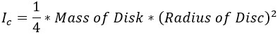
To approximate the disk inertia:

Figure 3: Approximate disk inertia
Where:
Approximating Submerged Weight for the Swing Check Valve
You can use Archimedes' Principle to approximate the submerged disk weight:

Special Conditions
A check valve can have a Special Condition of None, Closed (stays closed or allowed to reopen in transient), or Open (stays open).


