Check Valve Modeling (English Units)
Check Valve Modeling (Metric Units)
Summary
This example models the closure of the check valve in three ways for a system pumping water uphill loses power to the pump. The check valve is near the pump discharge. Results will be graphed to illustrate pressure on each side of the check valve, and animation features will be used to show the system pressure profile after the valve is closed.
Topics Covered
-
Modeling a check valve and fluid velocity at valve closure
-
Observing the differences between check valve models
-
Creating a system pressure profile animation
Required Knowledge
This example assumes the user has already worked through the Beginner: Valve Closure example, or has a level of knowledge consistent with that topic. You can also watch the AFT Impulse Quick Start Video (English Units) on the AFT website, as it covers the majority of the topics discussed in the Valve Closure example.
Model File
This example uses the following file, which is installed in the Examples folder as part of the AFT Impulse installation:
Step 1. Start AFT Impulse
From the Start Menu choose the AFT Impulse 9 folder and select AFT Impulse 9.
To ensure that your results are the same as those presented in this documentation, this example should be run using all default AFT Impulse settings, unless you are specifically instructed to do otherwise.
Step 2. Define the Fluid Properties Group
-
Open Analysis Setup from the toolbar or from the Analysis menu.
-
Open the Fluid panel then define the fluid:
-
Fluid Library = AFT Standard
-
Fluid = Water (liquid)
-
After selecting, click Add to Model
-
-
Temperature = 70 deg. F
-
Step 3. Define the Pipes and Junctions Group
At this point, the first two groups are completed in Analysis Setup. The next undefined group is the Pipes and Junctions group. To define this group, the model needs to be assembled with all pipes and junctions fully defined. Click OK to save and exit Analysis Setup then assemble the model as shown in the figure below.
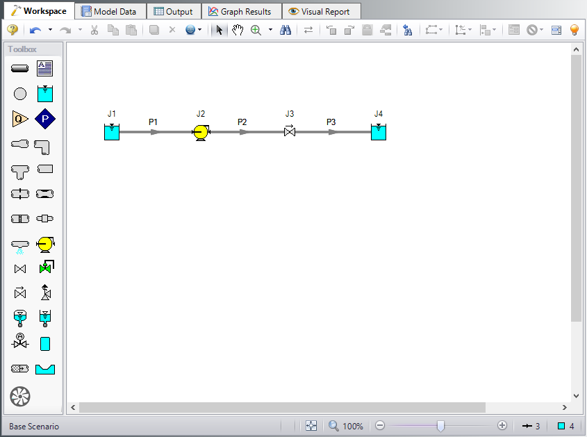
The system is in place but now we need to enter the input data for the pipes and junctions. Double-click each pipe and junction and enter the following data in the properties window.
For the first scenario, the simplest User Specified check valve type will be used. The Forward Velocity to Close Valve and Delta Head to Reopen should be obtained either from measured data, or from the data provided by the manufacturer. If no information is known, an estimate of 0 for both parameters may be used to represent an ideal check valve. However, a velocity to close of zero is not realistic, and should not be used for final engineering estimates. A more conservative engineering estimate would be achieved if some reverse flow is allowed through the check valve before it fully closes.
Pipe Properties
-
Pipe P1
-
Pipe Material = Steel - ANSI
-
Size = 8 inch
-
Type = STD (schedule 40)
-
Friction Model Data Set = Standard
-
Length = Use table below
-
| Pipe | Length (feet) |
|---|---|
| 1 | 10 |
| 2 | 10 |
| 3 | 1000 |
Junction Properties
-
Reservoir J1
-
Name = Lower Reservoir
-
Liquid Surface Elevation = 10 feet
-
Liquid Surface Pressure = 100 psig
-
Pipe Depth = 10 feet
-
-
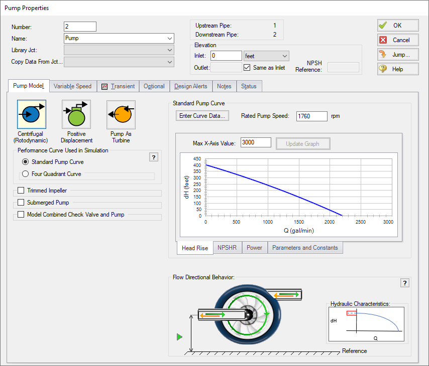
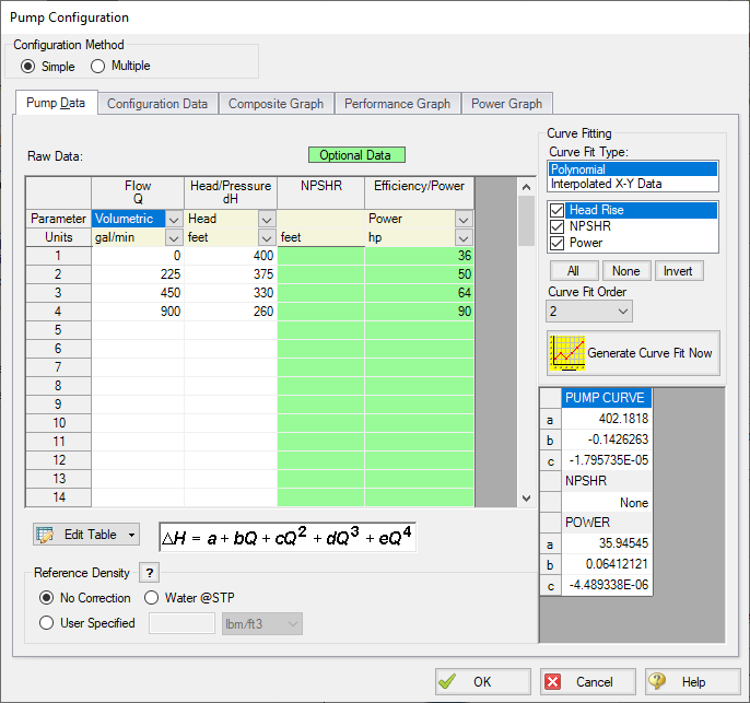
Pump J2
| Volumetric | Head | Power |
|---|---|---|
| gal/min | feet | hp |
| 0 | 400 | 36 |
| 225 | 375 | 50 |
| 450 | 330 | 64 |
| 900 | 260 | 90 |
-
Curve Fit Order = 2
-
Transient tab (Figure 4)
-
Transient = Trip
-
Transient Special Condition = None
-
Initiation of Transient = Single Event
-
Event Type = Time Absolute
-
Condition = Greater Than or Equal To
-
Value = 0 seconds
-
Total Rotating Inertia = User Estimated
-
Value = 25 lbm-ft2
-
-
Check Valve J3
-
Inlet Elevation = 0 feet
-
Valve Model = User Specified
-
Loss Model = Cv
-
Full Open Cv = 1515
-
Forward Velocity to Close Valve = -0.2 feet/sec
-
Delta Pressure/Head to Reopen = Pressure
-
Delta Pressure = 0 psid
-
-
Reservoir J4
-
Name = Upper Reservoir
-
Liquid Surface Elevation = 295 feet
-
Liquid Surface Pressure = 100 psig
-
Pipe Depth = 10 feet
-
Note: Unless specified otherwise, pipe elevation is assumed to vary linearly between junctions. Therefore, the pipe P2 inlet elevation is 0
ØTurn on the Show Object Status from the View menu to verify if all data is entered. If so, the Pipes and Junctions group in Analysis Setup will have a check mark. If not, the uncompleted pipes or junctions will have their number shown in red. If this happens, go back to the uncompleted pipes or junctions and enter the missing data.
Step 4. Define the Pipe Sectioning and Output Group
ØOpen Analysis Setup and open the Sectioning panel. When the panel is first opened it will automatically search for the best option for one to five sections in the controlling pipe. The results will be displayed in the table at the top. Select the row to use one section in the controlling pipe.
Step 5. Define the Transient Control Group
ØOpen the Simulation Mode/Duration panel in the Transient Control group. Enter 30 seconds for the Stop Time.
Navigate to the Transient Cavitation panel and select Discrete Gas Cavity Model, the default values that populate will suffice for this example.
All groups should now be complete and the model is ready to run. If all groups in Analysis Setup have a green checkmark then Click OK and proceed. Otherwise, enter the missing information.
Step 6. Run the Model
Click Run Model from the toolbar or from the Analysis menu. This will open the Solution Progress window. This window allows you to watch the progress of the Steady-State and Transient Solvers. When complete, click the Output button at the bottom of the Solution Progress window.
Step 7. Examine the Output
In the Output window there will be a warning shown stating that reverse flow occurs at the pump. If there is a high magnitude of reverse flow at the pump or the reverse flow occurs for a long duration, then we might want to update the pump to use four quadrant data. In this model the magnitude and duration of reverse flow is relatively small, so this warning will be dismissed.
Often when a check valve is present downstream of the pump reverse flow will be negligible and reverse flow warnings can be dismissed; However, it is always good practice to check the volumetric flow rate results at the pump to confirm. The Selecting a Pump Four Quadrant Curve example provides more information on how to perform a sensitivity analysis with four quadrant data if reverse flow is significant at the pump.
Now go to the Graph Results window by clicking the Graph Results tab.
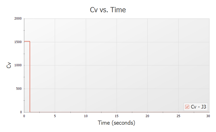
A. Graph the check valve Cv
To confirm the check valve's behavior create a plot of the check valve Cv over time as follows:
-
Select the Transient Jct tab in the Graph Parameter section
-
Add J3 (Check Valve) to be graphed
-
Make sure Check Valve Cv is the Parameter to graph
-
Click Generate
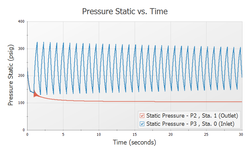
The check valve Cv plot can be seen in Figure 5 below. As is shown in the plot, the check valve closes instantly at about one second, which is the time when the velocity reaches zero at the check valve. The exact closure time can be seen in the Output window by selecting the Event Messages tab in the top third of the window. To model a slower closure a different check valve model will need to be chosen. This will be shown later in the example.
ØRight click on the graph and select Add Graph to List. Name this graph Check Valve Cv. Your graphing parameters will be saved to the Graph List Manager in the top right corner of the Graph Results Window. This enables you to quickly graph these same parameters in different scenarios. We will create scenarios for comparison later in this example.
B. Graph the transient pressures at the check valve
-
Still on the Graph Results window, go to the Transient Pipe tab, add the Pipe 2 Outlet and Pipe 3 Inlet. These represent each side of the check valve.
-
Make sure the selected parameter is Pressure Static.
-
Set the units to
-
Click Generate.
The resulting pressure transients are shown in Figure 6. It should be shown that after the valve closes, pressure between the pump and the check valve is brought to equilibrium while pressure after the check valve will experience water hammer. The maximum and minimum values can be shown by the Show Cross Hair tool in the Graph Results toolbar.
ØRight click on the graph and select Add Graph to List. Name this graph Check Valve Inlet/Outlet Pressure.
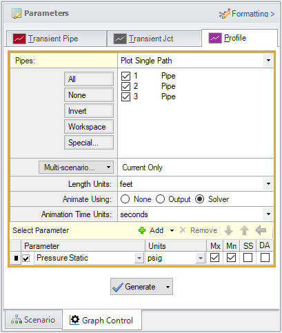
C. Graph the pipeline transient pressure profile
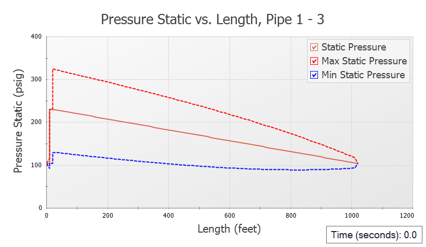
This animation will illustrate the static pressure throughout the pipe system over time.
-
Select the Profile tab on the Quick Access Panel (Figure 7).
-
In the Pipes area click All to select pipes 1-3.
-
Animate Using: Solver
-
In the Parameter area make sure Pressure Static is selected.
-
For units select
-
Click Generate.
Once the graph has been generated, press the Play button on the Graph Results animation controls as is shown in Figure 8 to observe how the pressure profile varies over time. At around 1 second the check valve closes, causing the maximum pressure spike observed in the system. The resulting pressure wave can then be seen moving along the pipe to the reservoir and being reflected back.
Right click on the graph and select Add Graph to List. Name this graph System Pressure Profile.
Step 8. Create Child Scenarios
Often the forward velocity to close and delta pressure to reopen the check valve are not directly known for the system as was shown above. However, data such as a reverse velocity vs deceleration chart, or information on the valve dimensions may be provided. In that case either the Estimate From Fluid Deceleration or Force Balance check valve model may be more appropriate.
The Estimate From Fluid Deceleration model type for a check valve requires that reopening is not possible. In order to model this scenario accurately, you will need valve performance data for the maximum reverse velocity vs fluid deceleration. If you model a valve with a preset that does not accurately represent your system, this could yield inaccurate results.
Modeling a check valve with the force balance model is ideal for either swing check valves or nozzle/plug check valves where you know the weight and dimensions of your check valve.
We will create scenarios to model each of the check valve types.
Open the Scenario Manager on the Quick Access Panel. Create a child scenario by right-clicking on the Base Scenario and then selecting Create Child. Do this four times, naming each one after the following check valve model types:
-
User Specified
-
Estimate from Fluid Deceleration - Dimensional
-
Estimate from Fluid Deceleration - Non-dimensional
-
Force Balance
Load the Estimate from Fluid Deceleration - Dimensional scenario by double-clicking the scenario name.
Step 9. Define and Run the Estimate from Fluid Deceleration Scenarios
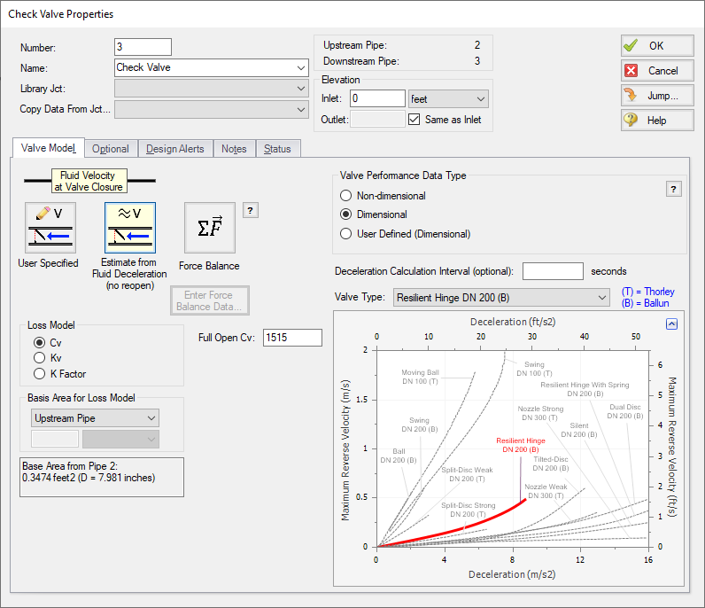
This modeling method is ideal for when you have Valve Performance Data / Fluid Deceleration to help define your check valve, or if you are using a check valve which is geometrically similar to the valves which have deceleration data provided in AFT Impulse (Figure 9). The valves from Ballun's data set were ANSI Class 125 size 8-inch valves. The data sets for Thorley were obtained using 4-inch and 12-inch valves. For more information on the test setups used by Ballun and Thorley see the check valve topic in the main help file.
A. Define the Estimate from Fluid Deceleration - Dimensional Scenario
Open J3 Check Valve properties window. Under Fluid Velocity at Valve Closure select Estimate from Fluid Deceleration (no reopen), as shown in Figure 9.
There are several Valve Performance Data Type options which can be selected. If you have a Deceleration vs Maximum Reverse Velocity chart provided by the valve manufacturer, the User Defined option should be selected, and the data entered. Otherwise, one of the data sets provided by Impulse can be used with either the Non-dimensional or Dimensional option. The dimensional option should be used if the valve in your system is similar in both geometry and size to the data set valve type. If your valve has similar geometry but is a different size than the valves tested to obtain the data set, then the Non-dimensional option should be used.
The dimensional model is applicable for this example because the check valve being modeled is an 8-inch swing-flex check valve, which is similar in both geometry and size to the Resilient Hinge DN 200 check valve used in the Ballun data set.
Define the check valve as follows:
-
Valve Performance Data Type = Dimensional
-
Valve Type = Resilient Hinge DN 200 (B)
B. Define the Estimate from Fluid Deceleration - Non-dimensional Scenario
Load the Estimate from Fluid Deceleration - Non-dimensional scenario by double-clicking the scenario name in the Scenario Manager.
Define the check valve as follows:
-
Fluid Velocity at Valve Closure = Estimate from Fluid Deceleration (no reopen)
-
Valve Performance Data Type = Non-dimensional
-
Minimum Velocity Required to Fully Open Valve (Vo) = 6.5 feet/sec
-
Valve Type = Resilient Hinge (B)
Note that there is a new parameter which is required to be entered when the non-dimensional valve type is used, the Minimum Velocity Required to Fully Open Valve (Vo). The Vo can be calculated through testing, or by consulting the valve manufacturer. For the purpose of this example the Vo was obtained by using the dimensional and non-dimensional deceleration charts provided by the manufacturer.
C. Run and Compare Results
Run the two Estimate from Fluid Deceleration scenarios and go to the Output window. Note that a warning is once again given for reverse flow at the pump. We will again dismiss this warning as the magnitude of reverse flow is low.
Next go to the Graph Results window. Regenerate each of the graphs for this scenario using the Graph List items by double-clicking the graph names in the Graph List Manager.
Notice that using the given information for the check valve these two models produce practically identical results to the user specified check valve model, since the check valve closes at a reverse velocity of about
Similar to the user specified model, the Estimate from Fluid Deceleration valve model closes the valve instantaneously once the calculated forward velocity to close has been reached. However, unlike the User Specified valve model, the fluid deceleration option will never allow the check valve to reopen, so this option should be used carefully.
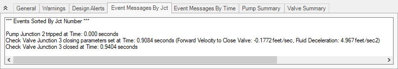
Figure 10: The Event Messages tab provides additional information on the fluid deceleration calculations at the check valve. The non-dimensional case is shown here
Step 10. Define the Force Balance Scenario
This modeling method is useful when you have information on the dimensions of the check valve in your system. This information may be available from the valve manufacturer, though in many cases it must be approximated. You can model swing check valves or translating nozzle check valves with the Force Balance method.
For this example we will use approximations of the valve dimensions from a schematic provided by the manufacturer to model the 8-inch Resilient Hinge swing check valve.
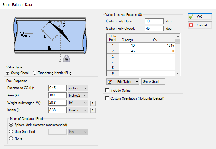
A. Enter the Check Valve Properties Data
Double click on J3 Check Valve.
-
Fluid Velocity at Valve Closure = Force Balance
-
Enter Force Balance Data =
-
Valve Type = Swing Check
-
Distance to CG (L) = 6.45 inches
-
Area (A) = 108 inches2
-
Weight (submerged, W) = 20.6 lbf
-
Inertia (I) = 8.38 lbm-ft2
-
Mass of Displaced Fluid = Sphere (disk diameter, recommended)
-
Note: Equations to approximate the submerged weight and inertia of the disk can be found in the AFT Impulse Help file, accessed from the ? buttons.
-
θ when Fully Open = 10 deg
-
θ when Fully Closed = 45 deg
-
Valve Loss vs. Position (θ) =
| θ (deg) | Cv |
|---|---|
| 10 | 1515 |
| 45 | 0 |
Note: For this example the Valve Loss vs. Position (θ) profile was assumed to be linear. For a more realistic force balance detailed information should be obtained and entered for the Cv profile from the valve manufacturer.
B. Run and Compare Results
Run the model and go to the Graph Results window.
Regenerate the pressure Check Valve Inlet/Outlet Pressure graph, as can be seen in Figure 12. Compared to the other three scenarios, the force balance check valve closure produces slightly larger pressure oscillations, with the amplitude of the oscillations increased by about
It can be seen from the check valve Cv graph (Figure 13) which displays the first 1.5 seconds of the run, that the check valve does not close over a single time step like in the previous scenarios, but instead closes rapidly over 1 second. Using a realistic Cv profile for the force balance input will allow for the most realistic calculation of this closing profile.
A comparison of the velocity at the check valves over the first 1.5 seconds can be seen in Figure 14. From the velocity graph it can be seen that the force balance check valve calculated a maximum reverse velocity of about
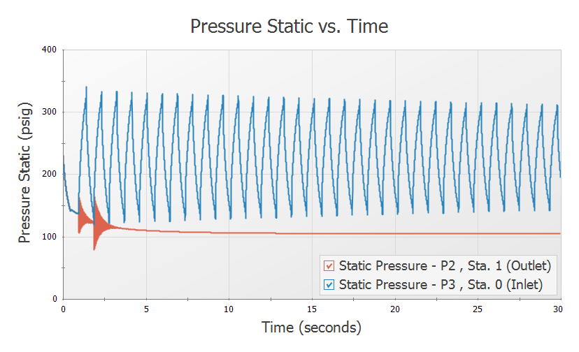
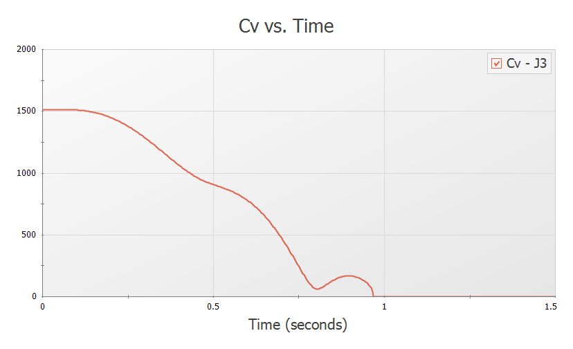
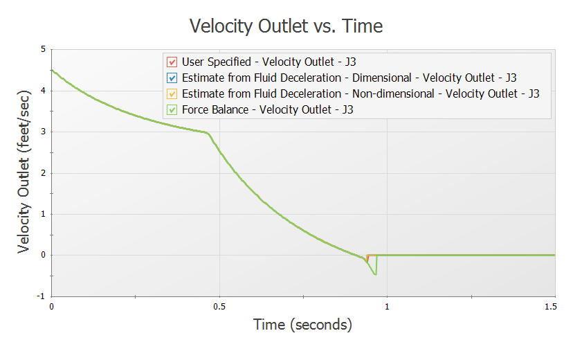
Figure 14: Velocity at the check valve outlet for each of the check valve types plotted for the first 3 seconds
Summary
Check Valves can be modeled in multiple ways depending on the information you have available to you. They can be modeled as combined with the pump outlet, with user specified fluid velocity, with estimated fluid velocity from fluid deceleration data, or with a force balance calculation. With enough reliable data, you should be able to get similar results with any modeling method.


