Selecting a Pump Four Quadrant Curve (English Units)
Selecting a Pump Four Quadrant Curve (Metric Units)
Summary
During waterhammer analysis of pumping systems there is potential for the pump to operate outside of its normal operating region where flow, head, and speed are positive. It may be required to use a four quadrant pump curve in order to better predict the pump’s behavior when operating outside of this normal operating region. As manufacturers rarely provide four quadrant data for the pump being used, a published four quadrant data set in dimensionless form is often chosen instead and dimensionalized to approximate the behavior of the actual pump being used in the system. For many cases the choice of four quadrant curve has a low impact on the waterhammer analysis results; however, this will not always be the case. This example is intended to provide the engineer with a deeper understanding of how to select four quadrant data sets for a waterhammer analysis, and how to evaluate the transient results predicted by the four quadrant curves.
This example considers a water transfer system for which several pump trip/valve closure cases are being modeled. There is a high possibility for reverse flow through the pump and reverse rotation of the pump impeller as the water is being pumped uphill, thus four quadrant data sets will be considered to model the behavior of the pump when operating with reverse flow and/or reverse rotation.
For those more interested in a quick how-to discussion and do not need in-depth discussion, consult the Overview of performing a sensitivity study for four quadrant analysis topic in Step 2 below.
Topics Covered
-
Selecting a four quadrant data set to analyze cases with reverse flow and/or reverse rotation at the pump
-
Performing sensitivity studies to assess four quadrant data selection
-
Comparison of the Best Efficiency Point (BEP) and Steady State Operating Point (SSOP) dimensional reference point options
Required Knowledge
This example assumes the user has already worked through the Beginner: Valve Closure example, or has a level of knowledge consistent with that topic. You can also watch the AFT Impulse Quick Start Video (English Units) on the AFT website, as it covers the majority of the topics discussed in the Valve Closure example.
This example expands on the topics introduced in the Pump Trip with Backflow - Four Quadrant Modeling example. It is recommended to work that example first as an introduction to basic four quadrant modeling concepts before working this example.
Nomenclature
As this is an advanced topic, a brief list of abbreviations is given here for reference.
| BEP | Best Efficiency Point of the standard pump curve |
| DRP | Dimensional Reference point, reference point used to create a four quadrant curve for a chosen four quadrant data set |
| Ns | Specific speed for the pump |
| SPC | Standard pump curve – sometimes called here the Manufacturer Curve, this is the head and efficiency (or power) vs. flow rate curve for the actual pump in your system |
| SSOP | Initial steady state operating point for the actual pump (from the manufacturer’s curve and system curve) |
| 4QBEP | Four quadrant pump curve created with reference to the BEP |
| 4QSSOP | Four quadrant pump curve created with reference to the SSOP |
Model Files
This example uses the following files, which are installed in the Examples folder as part of the AFT Impulse installation:
Step 1. Start AFT Impulse
From the Start Menu choose the AFT Impulse 9 folder and select AFT Impulse 9.
To ensure that your results are the same as those presented in this documentation, this example should be run using all default AFT Impulse settings, unless you are specifically instructed to do otherwise.
Step 2. Open the Model
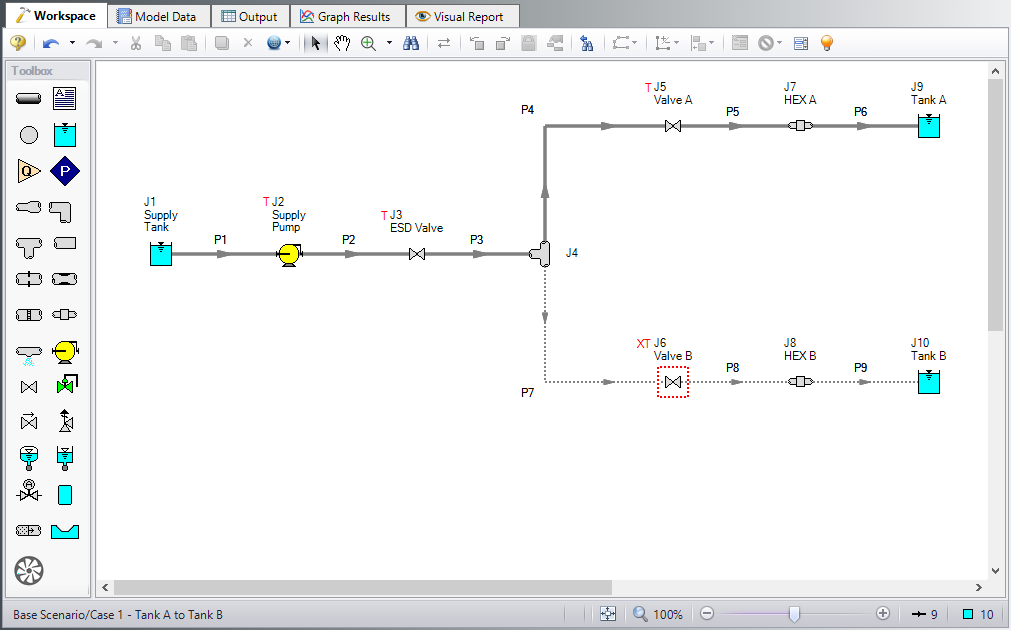
Water is being provided to two different processes, represented by Tank A and Tank B, as can be seen in Figure 1. The system is designed to provide water to one tank at a time.
In this transfer system several pump trip scenarios will need to be analyzed which have potential to experience back flow through the pump before the emergency shut-down (ESD) valve fully closes. Different four quadrant data sets will be compared against the manufacturer pump curve data for each of these cases to help the engineer understand the sensitivity to four quadrant data set selection and the range of potential predictions that result. The cases are as follows:
-
Unplanned pump trip after the flow has been transitioned from Tank A to Tank B
-
The pump operates far below BEP initially (about 60% BEP). Minimal reverse flow occurs at the pump.
-
-
Unplanned pump trip after the flow has been transitioned from Tank B to Tank A
-
The pump operates above BEP initially (about 113% BEP). Sustained reverse flow and reverse rotation occur at the pump.
-
-
Planned pump trip and Valve B closure after Valve A fails open
-
The pump operated at BEP initially. Sustained reverse flow and rotation occur at the pump.
-
Note: No pump startup cases are considered for this example, but the procedure is applicable to those situations as well if reverse flow does not occur during the initial steady state solution.
We will start with a given model file that is fully defined for the transient run using the manufacturer's curve. Navigate to the Examples folder installed with AFT Impulse, and open the model file named US - Selecting a Pump Four Quadrant Curve - Initial.imp to the Case 1 - Tank A to Tank B scenario.
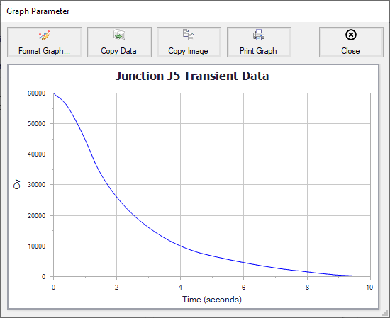
Note that we have four junctions with transients defined, as is denoted by the red T in the Workspace. These transients occur as two events. For the first event a planned switch from Tank A to Tank B occurs at time zero. Valve A will begin closing over ten seconds, following the transient shown in Figure 2 below. Valve B will begin opening at the same time over ten seconds following the reverse profile of that shown for Valve A. The second event happens twenty seconds into the transient run (ten seconds after the tank transition finishes), at which time an unplanned pump trip occurs and the ESD valve begins to close over seven seconds. The pump is modeled as a pump trip with inertia.
Step 3. Understand the Need for Sensitivity Studies for Four Quadrant Analysis
When the Standard Pump Curve is used (i.e., not four quadrant data) and reverse flow occurs at a pump, AFT Impulse uses the zero flow value for head and power. On a graph of head vs flow this would be represented as a horizontal line for negative flows. This may be a good estimate for negative flow that either has a small magnitude or happens for a short duration, but using a four quadrant data set is often better for high magnitude or sustained reverse flow, as this method introduces less uncertainty than just assuming that head and power would remain constant. Different four quadrant data sets can produce widely varied results, so choosing the four quadrant data set which best fits the pump being modeled is important.
Considerations for Choosing a Four Quadrant Curve
During the four quadrant data set selection process, there are several factors that will need to be accounted for. A brief background for each metric is provided below:
-
Pump Specific Speed: It is typically good practice to select a four quadrant data set based on the specific speed of the pump, as pumps with similar specific speeds will often behave similarly. However, the four quadrant data set with the closest reported specific speed is not always the best choice to represent the pump being analyzed for multiple reasons, including uncertainty in the accuracy of the reported specific speed for some four quadrant data sets. Thus, comparing multiple four quadrant data sets at specific speeds close to the specific speed of the pump being analyzed is advised. Note that in Impulse, each four quadrant data set is labeled as Preferred, Average, or Use With Caution, indicating the apparent quality of the four quadrant data set and the accuracy of the reported specific speed. When possible, the Preferred data sets should be selected for use in the model, as these sets provide the most trustworthy data. Average curves may be used if no Preferred data sets are available at similar specific speeds to the pump being used. The Use With Caution data sets should only be used when there are no Preferred or Average data sets that have a similar specific speed to the pump in use, or if the user has previous experience with using that data set which gives them confidence in that data set.
-
Comparison to Manufacturer’s Curve: The manufacturer's curve will always provide the most accurate prediction of the pump’s behavior while the pump is operating in the normal pumping zone of operation (i.e. flow in the positive direction, positive head, positive pump speed), and while the pump is operating within the range of flows that were tested by the manufacturer. Therefore it is reasonable to assume that a four quadrant data set which closely matches the manufacturer's curve while in the normal zone of operation will provide more accurate results than a four quadrant curve that shows larger differences from the manufacturer's curve in the normal pumping zone of operation. This comparison to the manufacturer's curve should be done for both the initial steady state operating point and the final operating point after all transients have died out. For this example we will refer to the final operating point after the transients have died out as the final steady state operating point. The reasoning for this will be discussed further throughout the example.
-
Dimensional Reference Point (DRP): Four quadrant data is usually published as a dimensionless set of data to allow it to be used for analysis with pumps besides the test pump. When dimensionalizing the data set for a pump, either the BEP or the SSOP may be used as the dimensional reference point. Many published four quadrant data sets use the BEP as the DRP to non-dimensionalize the data, so it seems logical that the BEP should be used as the DRP for the reverse transformation. However, if the pump is operating far from the BEP in the steady state, the initial steady state operating point predicted using the BEP as a DRP may be very different from the SSOP predicted from the manufacturer's curve. In that case using the SSOP as the DRP is useful to prevent differences from the steady state results using the manufacturer’s curve. However, using the SSOP as the DRP often causes large differences between the manufacturer's curve and the four quadrant curve. In summary, there is often a trade-off between how well the four quadrant curve matches the manufacturer’s curve for the steady state and final steady state, so it is always advised to test both DRP options. Note that if the simulation begins with a significantly incorrect initial flowrate, this will impact all subsequent results in a way that may be difficult to assess.
Procedure for Comparing Four Quadrant Data Sets
-
To perform the sensitivity study explained above the following steps can be taken:
-
Create a child scenario of the scenario that is defined using the manufacturer's curve
-
Open the Pump Properties window and select Four Quadrant Curve as the Performance Curve Used in Simulation
-
Choose User Selected and click Specify Model to launch the Specify Four Quadrant Model window
-
Choose the desired four quadrant data set from the drop-down list at the top of the window, and select Best Efficiency Point as the Dimensional Reference Point.
-
Select OK to accept the changes
-
Clone the current scenario and change the Dimensional Reference Point to the Steady-State Operating Point in the cloned scenario
-
Repeat steps 1 - 6 for each data set to be analyzed
-
Run all of the newly created scenarios and compare the transient results. Note that frequently results will not differ greatly among scenarios. In that case, results are not very sensitive to the specific choice of four quadrant curve. This makes the analyst’s job easier.
-
In order to be most conservative, use the worst case predictions from among the various four quadrant scenarios for design purposes.
-
If the worst case predictions lead to excessive and/or expensive implications in design and/or operations, take a closer look at results. Compare each four quadrant pump curve to the manufacturer’s curve at the initial steady state and, if applicable, the final steady state operating points to determine which scenario(s) appears to give the most accurate results. Criteria used to decide the most reliable four quadrant curve(s) include:
-
Similarity of specific speed, Ns – when making this comparison, be sure you have an accurate Ns value for your pump (see discussion below for more on this)
-
Overall agreement between the manufacturer’s curve (Standard Pump Curve) and dimensionalized four quadrant curve for head and power vs. flow rate in the normal zone of pump operation (Impulse displays these curves for you – review the comparisons)
-
Give more weight to the four quadrant curves which show closer agreement within the range of flow rates that the manufacturer tested the pump at (i.e. the range of flow rates that the pump curve is graphed for on the specification sheet)
-
Give more weight to four quadrant curves which generate transient results similar to the Standard Pump Curve during time frames when the pump is operating in the normal zone of operation
-
Give more weight to four quadrant curves Impulse categorizes as Preferred
-
Good agreement in initial steady-state flow rates between SPC and four quadrant curve
-
Good agreement in final steady-state flow rates between SPC and four quadrant curve – this not as important as agreement in initial steady-state flow rates, but should be considered
-
Note that there are several reasons why the engineer may choose to skip Step 10 above. One reason would be if the transient results for the different scenarios show only minor differences as noted in step 8 above. In that case it would be unnecessary to determine which scenario is most accurate, as any scenario will produce similar results. Another reason would be if the engineer’s analysis involves a project where highly conservative results are required, such as for a nuclear system. In that case the engineer could choose to simply use the most extreme results for the analysis for their design purposes. Note this means that if different scenarios produce the worst-case pressures in different areas of the model, then the engineer may want to use the most extreme results (e.g., highest or lowest pressure) regardless of scenario, rather than only using the results from one scenario.
Step 3. Run the Model with the Manufacturer's Curve
ØClick Run Model from the Toolbar or Analysis menu, then proceed to the Output window.
Notice that two warnings are given for this scenario, one indicating that negative head rise was calculated at the pump, and one indicating that reverse flow occurred at the pump. It will be easier to discuss these warnings by reviewing the transient head rise and flow rate at the pump.
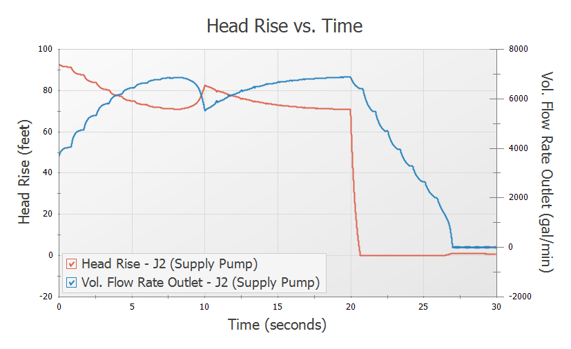
ØGo to the Graph Results window. In the Graph List Manager on the Quick Access Panel double click the Head Rise and Vol Flow at Pump Outlet graph list item to load the graph shown in Figure 3. You should see that the flow rate remains positive for the majority of the transient, with minor reverse flow occurring after 27 seconds, never reaching a magnitude higher than 30 gal/min. Graphing the pump head rise shows that the head rise reaches zero at about 21 seconds, and is fixed at zero until around 27 seconds. The low magnitude of reverse flow would suggest that a four quadrant curve may not be needed for use in this model. However, the head rise results introduce a large amount of uncertainty into the results, since AFT Impulse artificially fixes the head rise to zero. Using a four quadrant curve will allow Impulse to estimate the negative head rise which would occur at the actual pump.
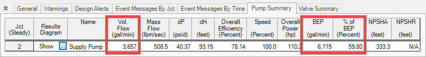
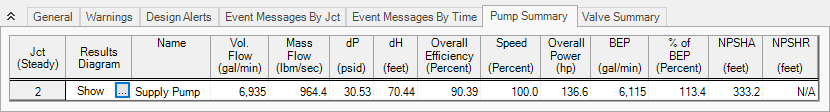
ØReturn to the Output window and go to the Pump Summary tab (Figure 4). The BEP was calculated based on the user-specified power curve to be
Step 4. Choose Four Quadrant Data Sets to Analyze
A. Calculating or Estimating Specific Speed
From the first consideration above, the first step for selecting the four quadrant curve will be to determine the specific speed of the pump and choose a four quadrant data set accordingly. AFT Impulse has a built-in tool to estimate the specific speed for the pump on the Specify Four Quadrant Model window if the specific speed is not available from the manufacturer.
ØCreate a child scenario of Case 1 - Tank A to Tank B named Manufacturer's Curve, this scenario will hold the results that were just obtained. Create another child of the Case 1 - Tank A to Tank B scenario named Four Quadrant Curve. Next, open the Pump Properties window. Select Four Quadrant Curve, choose User Specified for the type, then click Specify Model. By clicking Suggest a Data Set towards the top of the window, we can see that Impulse has estimated a specific speed of
The first assumption involves the impeller size for the pump. ANSI/HI 14.3.1.3.1-2019 states that the specific speed for any pump should be calculated for the pump at the maximum impeller size. Impulse will assume by default that the pump is untrimmed. However, for this example the impeller was trimmed. The specific speed estimate in Impulse can be improved by entering the trimmed and untrimmed impeller sizes, allowing Impulse to adjust the head and flow values using the affinity laws.
ØSelect Trimmed under Impeller Diameter, and enter
Another assumption contributing to this discrepancy involves the flow rate used for the calculation. ANSI/HI 14.3.1.3.1-2019 states that the specific speed should be calculated using the total flow through the pump. However, the standard does note that there is an alternate definition in industry which defines the specific speed as the flow rate per impeller eye. For double suction pumps (such as the pump in this example) this definition produces a specific speed which is reduced by 1/sqr(2), or approximately 0.707 times the total flow definition. If the specific speed value provided by the manufacturer (
ØChoose Select Suggested Data Set and Close to accept the suggested
Note: In cases like this where the specific speed has been provided by the manufacturer the value provided by the manufacturer will typically be more accurate. However, the engineer should verify whether the manufacturer has reported the specific speed based on the total flow or flow per impeller eye.
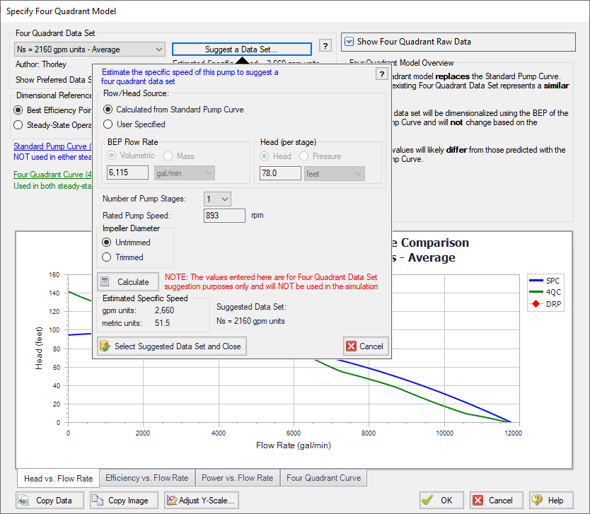
Figure 5: Impulse can estimate the specific speed and suggest the nearest four quadrant data set in the Specify Four Quadrant window. Suggested Data sets will by default only be Preferred or Average
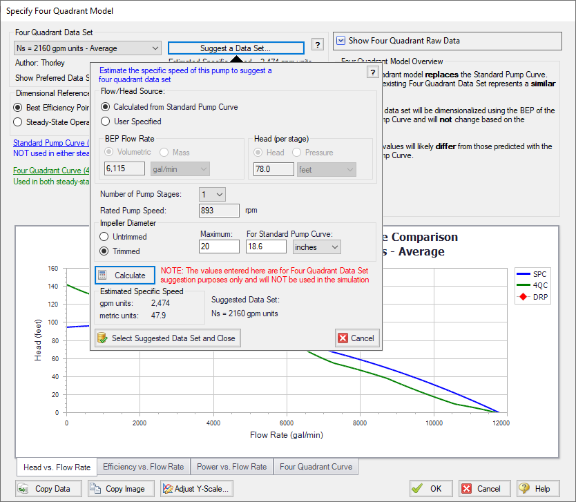
Figure 6: Impulse can account for trimmed impeller pumps using the affinity laws to adjust the flow rate and head for calculations, as shown above
B. Setting up Four Quadrant Scenarios
We just determined that the four quadrant data set with the closest specific speed is the
Each of the selected data sets should now be compared to the manufacturer's curve with the data set dimensionalized at the BEP and the SSOP. From here on we will refer to four quadrant curves that have been dimensionalized using the BEP as 4QBEP curves, and four quadrant curves that have been dimensionalized using the SSOP as 4QSSOP curves for convenience.
Create the scenarios for the selected four quadrant data sets as follows:
-
In the current Four Quadrant Curve Scenario check that BEP is selected for the DRP (dimensional reference point). Note that the head, efficiency, and power curves versus flow can be seen plotted against the Standard Pump Curve (referred to as the manufacturer’s curve for this example) at the bottom of this window, as shown below for head in Figure 7 and power in Figure 8.
Note: The raw data from the graphs shown in the Specify Four Quadrant Model window (Figure 7 and Figure 8) can be copied using the Copy Data button at the bottom of the window to compare this data for all scenarios in Microsoft Excel.
-
Select OK to accept the current settings.
-
Rename the Four Quadrant Curve scenario in the Scenario Manager as
-
Clone the
-
Create cloned scenarios for the
-
Run all of the four quadrant scenarios so that they have results.
Note: A batch run can be used to speed up the process of running multiple scenarios. This can be set up from the File menu by selecting Start Batch Run, then selecting all of the scenarios to be run and clicking Start Run.
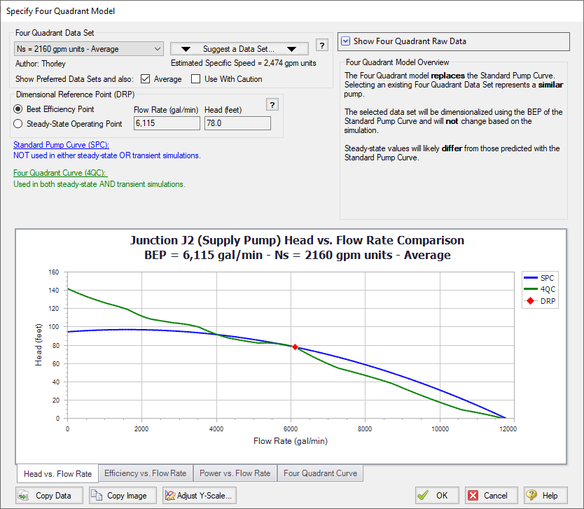
Figure 7: Specify Four Quadrant window showing the Head vs Flow data for the Ns =
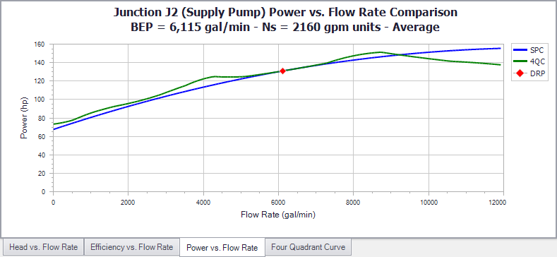
Figure 8: Power vs Flow graph from the Specify Four Quadrant window for the Ns =
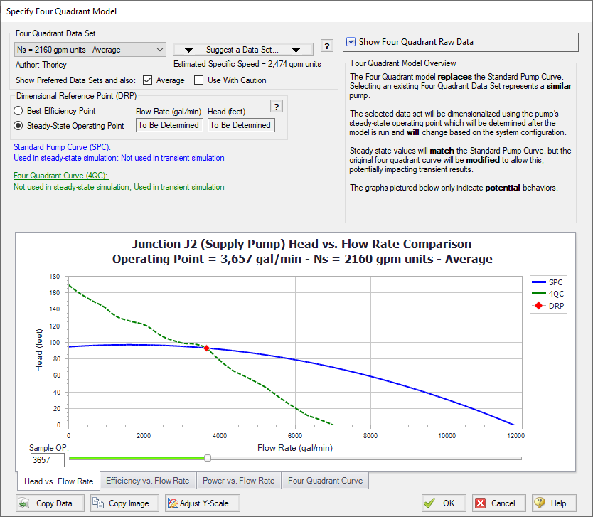
Figure 9: Specify Four Quadrant window showing the Head vs Flow data for the Ns =
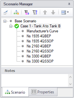
Figure 10: Scenario Manager with the scenarios created for each of the four quadrant data sets dimensionalized at the BEP and SSOP
C. Comparing Four Quadrant Pump Curves
If the engineer’s goal is simply to perform the most conservative analysis possible in the shortest amount of time, then comparing the pump curves as will be done below would be unnecessary. Instead, the engineer should simply proceed to compare the transient results for all four quadrant scenarios and use the maximum/minimum results from all cases, as was discussed at the beginning of this example.
Additionally, the below comparison may prove to be unnecessary if the transient results show negligible differences. However, we will compare the manufacturer’s curve and four quadrant pump curves here to be thorough.
Finding the actual initial and final steady state flow rates
For the next step in the sensitivity analysis we will compare all of the pump curves to the manufacturer’s curve at both the initial steady state operating point and the final steady state operating point, as was mentioned at the beginning of this example. There are two transient events that occur in this model, so in a sense we have two final operating points, one after each event. The final operating point for Event 1 will be when the flow has fully transitioned to Tank B, but Event 2 has not yet begun. The final operating point for Event 2 will be when the ESD valve and Valve A have fully closed, preventing flow in the system. We need to compare the four quadrant curves for the final operating point after Event 1, since the operating point at this time will affect the results for Event 2. After Event 2 the system will be at zero flow and no transients will occur, so this is not a point of interest for comparison.
The initial and final steady state flow rates can be found by running the manufacturer’s curve scenario, as was done earlier in the example. In this case we already saw that the steady state operating point for the pump was
Checking the dimensionalized curves
Each individual four quadrant curve can be compared to the manufacturer’s curve within the Specify Four Quadrant Model window in Impulse, as was seen above in Figure 7 and Figure 8 for the
When the BEP is used as the dimensional reference point, there is only one possible effective head and power curve for each four quadrant data set, as the BEP will not change when the system changes. However, if the steady state operating point is chosen then different effective head and power curves for each four quadrant data set will result depending on where the manufacturer’s curve operates during the initial steady state. Use the slider or the text box on the graph in the Specify Four Quadrant Model window to make sure that the graph is displaying the four quadrant curve for the actual steady state operating point before using the graph for comparison. The
If any four quadrant data set shows a substantial discrepancy for the initial or final steady state operating point, then it may be prudent to consider substituting this data set for another, in particular if the data set you are inspecting is marked as Average or Use With Caution.
Pump vs System Curve Comparison
To more easily compare the curves, the operating points for the head curves are shown using a multi-scenario pump vs. system curve that was created in Fathom 12 (Figure 11). The power curves are graphed in Figure 12 using Microsoft Excel. Table 1 listing the operating points shown in Figure 11 is also provided below for convenience. An engineer would not typically need to do this, but it is shown here to help reinforce the concepts discussed.
Each of the 4QBEP head curves cross the manufacturer's curve at the BEP, which is
We should also compare the final system curve to the pump curves. The final steady state will impact any transients that may occur later on in the simulation or after the end of the simulation, such as a sudden valve closure. In this case the Final System Curve represents the steady state after the first event (Valve A closing and Valve B opening), but before the second event (the unplanned pump tripping while the ESD valve closes). Thus any large differences in the final steady state will impact the subsequent pump trip. It can be seen from Figure 11 below that each of the 4QBEP curves show deviations from the manufacturer's curve at the Final System Curve, but the 4QSSOP curves show a much larger deviation than the 4QBEP curves. The
In Figure 12 we can see similar trends to those observed for the power curves. At the initial steady state the 4QSSOP curves match the manufacturer’s curve perfectly, while the 4QBEP curves deviate by various amounts. Near the final steady state flow the 4QSSOP curves show significantly more deviation than the 4QBEP curves. This is likely due to the fact that the initial steady state flow is far from the final steady state flow.
The
Table 1: Pump head, flow, and discharge velocity at the initial and final steady state operating points as can be seen in Figure 11. The Manufacturer’s Curve shows the correct results, while the others are an artifact of the selected 4Q curve
|
|
Initial Steady-State | Final Steady-State | ||||
|---|---|---|---|---|---|---|
| Pump Curve | Flow (gal/min) | Head (feet) | Velocity (feet/sec) | Flow (gal/min) | Head (feet) | Velocity (feet/sec) |
| Manufacturer's Curve | 3,657 | 93.15 | 4.031 | 6,937 | 70.42 | 7.647 |
| 1935 4QBEP | 2,566 | 86.52 | 2.829 | 7,166 | 72.79 | 7.900 |
| 1935 4QSSOP | 3,657 | 93.15 | 4.031 | 5,465 | 57.14 | 6.025 |
| 2160 4QBEP | 3,835 | 94.44 | 4.228 | 6,607 | 67.15 | 7.283 |
| 2160 4QSSOP | 3,657 | 93.15 | 4.031 | 4,917 | 53.00 | 5.420 |
| 3300 4QBEP | 4,320 | 98.25 | 4.763 | 6,740 | 68.45 | 7.430 |
| 3300 4QSSOP | 3,657 | 93.15 | 4.031 | 5,023 | 53.77 | 5.538 |
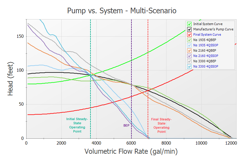
Figure 11: Pump vs. System Curve plot showing the manufacturer provided pump curve compared to pump curves from the
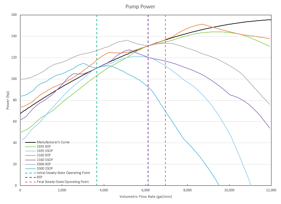
Figure 12: Pump Power Curve plot showing the manufacturer provided power curve compared to power curves from the
Step 5. Compare the Transient Results
We now want to compare the results to see how sensitive the results are to the choice of pump curve used for the simulation.
First go to the Output window for any of the four quadrant scenarios. Note that when any of the four quadrant scenarios are run, several information items will be given in the Warnings tab of the Output window. These messages are meant to inform the user of the potential implications that the four quadrant curves may have for the model, which this example explains in detail.
Now go to the Graph Results window and generate a graph of the pump speed and the velocity at the pump outlet, as can be seen in Figure 13 and Figure 14 below. From Figure 13 we can see that the pump does not reach zero speed during the transient simulation, meaning that the pump does not experience reverse rotation. In Figure 14 the velocity results at the outlet of the pump are compared. Recall from Step 3 that reverse flow occurs at the pump at around 27 seconds, though the magnitude of reverse flow was minor. In addition, during Step 3 we found that negative head rise would occur at the pump starting at 21 seconds. Since the pump operates at positive speed, positive flow and positive head for the first 21 seconds of the transient, the manufacturer’s curve will produce the most accurate results during this time. Therefore, the four quadrant curve results can be compared directly to the manufacturer’s curve results to determine the error in the four quadrant curve results up to 21 seconds into the transient run. After 21 seconds one of the four quadrant curves will likely give more accurate results.
For this case there is a clear difference between the initial steady state velocity (at time zero) using the manufacturer’s curve and the steady-state velocities using the
The static pressure at the ESD valve outlet is shown in Figure 15, with the maximum and minimum pressures detailed in Table 2. We can see that the maximum and minimum pressures at the ESD valve occur once the ESD valve has fully closed after 27 seconds. The 4QSSOP pressure results experience significantly decreased peak pressures and do not experience the low pressure peaks that are seen at about 27 and 28.5 seconds for the other Case 1 scenarios.
For example, consider the 2160 4QSSOP results, which we noted showed the largest difference in the velocity results when compared to the manufacturer’s curve at time 20 seconds. The 2160 4QSSOP curve has a maximum pressure of about 174 psia, as compared to the 238 psia peak pressure for the manufacturer’s curve (See Table 2 below). At about 27 seconds a low pressure of 80 psia is calculated using the manufacturer’s curve, while the 2160 4QSSOP curve remains at a pressure of 146 psia.
This difference in results makes sense based on the large differences from the manufacturer's curve at the final system curve, as were shown in Figure 11. Note for completeness that the Figure 11 final steady state values would compare most precisely to the Impulse results if the transient was run longer and the unplanned pump trip at 20 seconds did not occur. In other words, the waterhammer transients need to all die out for Impulse to find the true, final steady state. We can see in Figure 14 at 20 seconds that the transient velocity has roughly but not completely steadied out.
Overall for Case 1 where negligible reverse flow occurs at the pump, we can see that the large differences observed between the 4QSSOP curves and the manufacturer’s curve at the final steady state resulted in large variation in the results, especially for the pressures at the ESD valve outlet. The differences in the steady state results for the 4QBEP curves did not result in significant error in the transient results for this case due to the fact that the valve closures during the first transient event were not sensitive to the steady state results. In this case one of the 4QBEP curves would be the best choice out of the four quadrant curves analyzed as Case 1 is much more sensitive to the final steady state conditions (i.e., at 20 seconds before the pump trips) than it is to the initial steady state.
Table 2: Maximum and minimum static pressures at ESD valve and time at which the pressures occur for Case 1. Note that the results for the manufacturer’s curve are suspect after 21 seconds per the discussion above
|
|
Max. Static Pressure | Max. Static Pressure Time | Min. Static Pressure | Min Static Pressure Time |
|---|---|---|---|---|
| Pump Curve | psia | seconds | psia | seconds |
| Manufacturer's Curve | 233.8 | 27.85 | 85.92 | 27.02 |
| Ns 1935 4QBEP | 222.2 | 27.85 | 97.42 | 27.02 |
| Ns 1935 4QSSOP | 185.0 | 0.00 | 131.0 | 20.85 |
| Ns 2160 4QBEP | 218.2 | 27.85 | 101.4 | 27.02 |
| Ns 2160 4QSSOP | 185.0 | 0.00 | 139.7 | 21.70 |
| Ns 3300 4QBEP | 230.7 | 27.85 | 88.96 | 27.02 |
| Ns 3300 4QSSOP | 185.7 | 27.85 | 134.1 | 27.02 |
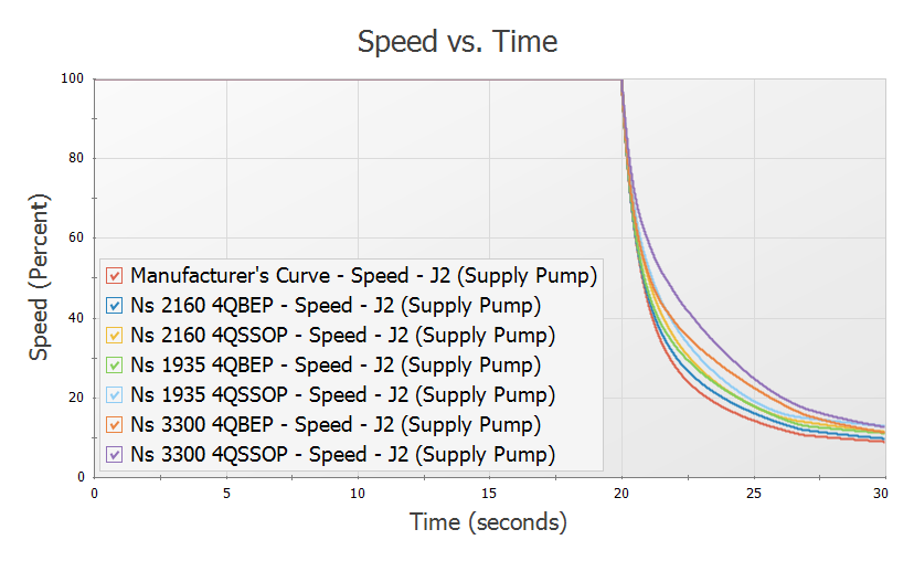
Figure 13: Pump speed vs time for Case 1 using the manufacturer's curve and each of the four quadrant curve scenarios
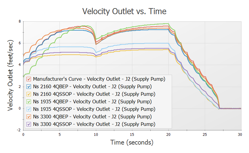
Figure 14: Velocity at pump outlet for Case 1 using the manufacturer's curve and each of the four quadrant curve scenarios
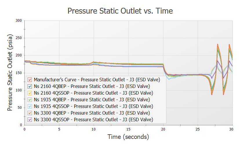
Figure 15: Static pressure at ESD Valve outlet for Case 1 using the manufacturer's curve and each of the four quadrant curve scenarios
Step 6. Case 2 - Tank B to Tank A
Case 1 operated in the normal pumping zone of operation (positive speed, head and flow) for the majority of the run, so four quadrant data was only required for the analysis of the results when the pump experienced negative head. Case 2 and Case 3 may experience more extensive negative flow, speed, and/or head at the pump requiring further use of four quadrant methods.
A. Create Scenarios for Case 2
For Case 2 the system starts with flow to Tank B during the steady state. The flow then transitions from Tank B to Tank A over ten seconds. At twenty seconds into the transient, the pump trips and the ESD valve closes, as occurred in Case 1.
Let's create scenarios for Case 2 and repeat the analysis above. Do the following:
-
Right-click the Case 1 - Tank A to Tank B scenario and select Clone With Children. Rename the scenario to Case 2 - Tank B to Tank A
-
Open the Valve Properties window for Valve A (J5). We will need to set this valve to begin closed, and open over ten seconds.
-
On the Optional tab set the Special Condition to Closed
-
Go to the Transient tab. Under the Transient Data menu select Import from File from the drop-down menu, then browse to 10 Sec Valve Opening.txt in the Impulse Examples folder
-
Select Tab as the Separator, then click OK. The data should now start with Cv = 0 at time 0, and open to Cv = 6000 at 10 seconds
-
Now open the Valve Properties window for Valve B. This valve will need to begin open, then close over 10 seconds.
-
On the Optional tab set the Special Condition to None
-
Go to the Transient tab. Under the Transient Data menu select Import from File from the drop-down menu, then browse to 10 Sec Valve Closing.txt in the Impulse Examples folder
-
Select Tab as the Separator, then click OK. The data should now start with Cv = 60000 at time 0, and close to Cv = 0 at 10 seconds. The Cv vs. time data should be the same as shown earlier in Figure 2 for Case 1, Valve A.
B. Compare Four Quadrant Curves to Manufacturer's Curve
Now that the scenario is fully defined, let's examine the results for the model using the manufacturer's curve.
ØRun the Case 2 - Tank B to Tank A scenario from the shortcut on the toolbar, or from the Analysis menu, and go to the Output window.
There will be several warnings visible for this scenario. A warning is given for reverse flow at the pump. If we were to graph the flow rate at the pump as was done for Case 1 we would see that a significant magnitude of reverse flow occurs towards the end of the transient run, thus it would be wise to use four quadrant data for this case. This is discussed further in Step 6-C.
Warnings are also given that the static pressure is lower than the vapor pressure at several pipe stations. This warning is given because cavitation modeling was disabled in the Transient Control window in order to decrease the run time for this model. When cavitation modeling is disabled the pressure is allowed to drop below an absolute pressure of zero. Though this is not realistic, we will leave cavitation modeling disabled to simplify the model for the purpose of this example – as well as to better be able to see the impact on low pressures from different pump curve choices. This can be done as the cavitation in this model is minor and has a low impact on the pressure results. When modeling an actual system the cavitation modeling should be turned on in Transient Control in order to obtain more realistic results.
ØGo to the Pump Summary tab. For this case the pump is operating at
As was done in Step 4-C for Case 1, let's compare the manufacturer's pump curve to the dimensionalized four quadrant curves. It will again be useful to compare the pump curves to both the initial steady state, and the final steady state for the system after the tank transition and before the pump trips. Note that the final steady state for Case 2 will be equivalent to the initial steady state for Case 1, which means the final steady state operating point for Case 2 occurs at a flow rate of
A multi-scenario pump vs. system curve graph was generated in AFT Fathom for Case 2, as can be seen in Figure 17, with the operating points from Figure 17 shown in Table 3. The power curves for each of the scenarios can be seen in Figure 18.
In this case the pump operates much closer to BEP, resulting in fewer differences between the 4QSSOP curves and the 4QBEP curves. All of the four quadrant pump head curves intersect the initial steady state system curve close to the manufacturer's curve, though the 4QBEP curves do show minor differences in the steady state operating point. At the final system curve there is not a clear trend when comparing the 4QSSOP and 4QBEP curves. Instead the curves are grouped based on the specific speed, rather than dimensional operating point. Both
Another point of interest is that the
The comparison of the power curves again shows similar trends. In this case it is difficult to determine qualitatively which four quadrant data set best matches the manufacturer curve, though the
If looking for the most reliable four quadrant curve in this case, one of the 2160 data sets should be chosen due to the closer match that the 2160 curves show at the final steady state for the head and power curves. If the system is sensitive to the initial steady state then the 2160 4QSSOP curve should be chosen.
Table 3: Pump head, flow, and discharge velocity at the initial and final steady state operating points as can be seen in Figure 17
|
|
Initial Steady-State | Final Steady-State | ||||
|---|---|---|---|---|---|---|
| Pump Curve | Flow (gal/min) | Head (feet) | Velocity (feet/sec) | Flow (gal/min) | Head (feet) | Velocity (feet/sec) |
| Manufacturer's Curve | 6,935 | 70.44 | 7.645 | 3,658 | 93.14 | 4.033 |
| 1935 4QBEP | 7,165 | 72.79 | 7.899 | 2,566 | 86.56 | 2.829 |
| 1935 4QSSOP | 6,935 | 70.44 | 7.645 | -111 | 80.32 | -0.122 |
| 2160 4QBEP | 6,605 | 67.19 | 7.281 | 3,836 | 94.43 | 4.229 |
| 2160 4QSSOP | 6,935 | 70.44 | 7.645 | 3,617 | 92.85 | 3.987 |
| 3300 4QBEP | 6,738 | 68.48 | 7.427 | 4,321 | 98.24 | 4.764 |
| 3300 4QSSOP | 6,935 | 70.44 | 7.645 | 4,189 | 97.16 | 4.618 |
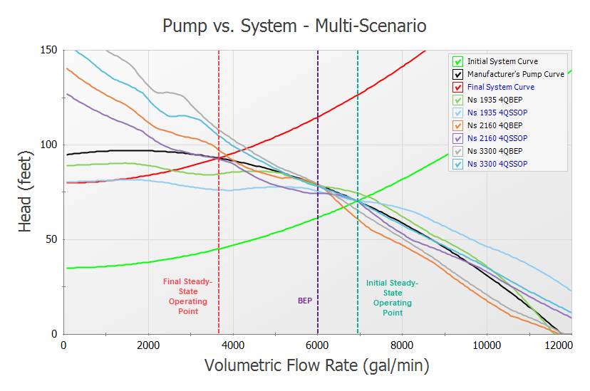
Figure 17: Pump vs. System Curve plot showing the manufacturer provided pump curve compared to pump curves from the
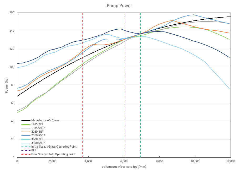
Figure 18: Pump Power Curve plot showing the manufacturer provided power curve compared to power curves from the
C. Examine Transient Results for Case 2
ØRun each of the four quadrant scenarios using the batch run feature from the file menu, then proceed to the Graph Results window.
From the pump speed and velocity graphs in Figure 19 and Figure 20 it can be seen that the pump will operate in the normal pumping zone of operation with both forwards flow and positive speed up until about 10 seconds into the transient. Depending on the pump curve being used, the pump experiences some reverse flow between 10 seconds and 27 seconds, though most (but not all) of the pump curve results return to forward flow before reversing again. From the pump speed curve we can see that all of the four quadrant curves predict that the pump will begin to operate at negative speeds (reverse rotation) between 24 - 26 seconds. This means that for the time period between 24 - 27 seconds the pump will likely operate with both reverse flow and rotation. There is a high level of uncertainty when using the manufacturer's curve due to the magnitude and duration of reverse flow and reverse rotation, so the manufacturer’s curve should not be used as a measure of accuracy once the flow becomes negative (at about 10 seconds), and especially during negative rotation.
Note: When the Standard Pump Curve option is used to model a pump in Impulse, the speed will not be allowed to go below 0%, similar to how the head rise was limited to a minimum of 0 in Case 1 when the SPC was used.
Further examining the velocity at the pump we can see that there is less deviation in the initial velocity for each of the curves. In this case this is due to the pump operating closer to the BEP than Case 1. However, the distribution of velocities is much broader once the tank transition has finished at around 10 seconds, reflecting the broader distribution we observed in the pump head curves.
Figure 21 shows the pressure results at the outlet of the ESD valve for the pump trip case, while Table 4 details the maximum and minimum pressures shown in the graph. The range of peak pressures predicted using the four quadrant curves at 27 seconds has been reduced from about
Zooming in on the minimum pressures that occur at about 28 seconds and 30 seconds into the run (shown in Figure 22) shows that
Be aware that the ESD valve pressures do not represent the overall maximum/minimum pressures for the system in this case. Many of the Case 2 scenarios actually reach vapor pressure at the outlet of Valve B, even the scenarios which did not drop to vapor pressure at the ESD valve. In an actual analysis the engineer would need to assess the impact of cavitation on the model and consider mitigation such as alternate valve closure times/profiles or installing protective equipment, though this will not be discussed further in this example.
To be conservative the engineer could simply choose the extreme case, which would be the
Table 4: Maximum and minimum static pressures at ESD valve and time at which the pressures occur for Case 2 as shown in Figure 21 and Figure 22 below. Note that minimum pressures below absolute zero are not physically possible but are shown for comparison purposes
|
|
Max. Static Pressure | Max. Static Pressure Time | Min. Static Pressure | Min Static Pressure Time |
|---|---|---|---|---|
| Pump Curve | psia | seconds | psia | seconds |
| Manufacturer's Curve | 394.4 | 27.01 | -33.79 | 27.85 |
| 1935 4QBEP | 379.1 | 27.01 | -18.69 | 27.85 |
| 1935 4QSSOP | 397.8 | 27.01 | -37.19 | 27.85 |
| 2160 4QBEP | 347.5 | 27.01 | -9.90 | 10.00 |
| 2160 4QSSOP | 360.0 | 27.01 | -9.07 | 10.00 |
| 3300 4QBEP | 349.0 | 27.02 | -13.93 | 10.00 |
| 3300 4QSSOP | 356.4 | 27.01 | -12.86 | 10.00 |
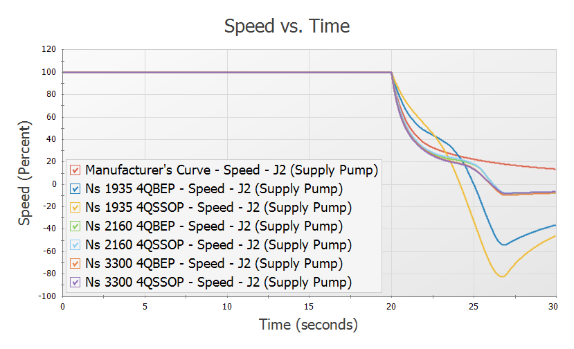
Figure 19: Pump speed vs time for Case 2 using the manufacturer's curve and each of the four quadrant curve scenarios
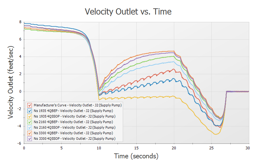
Figure 20: Velocity at pump outlet for Case 2 using the manufacturer's curve and each of the four quadrant curve scenarios
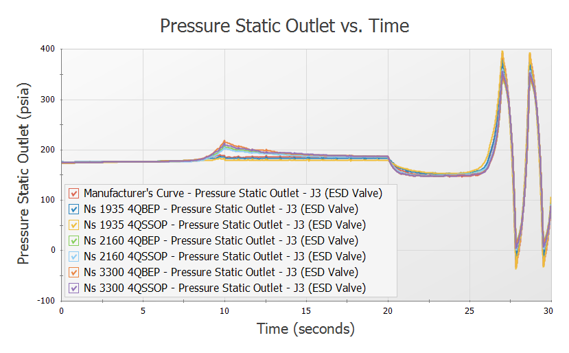
Figure 21: Static pressure at ESD Valve outlet for Case 2 using the manufacturer's curve and each of the four quadrant curve scenarios
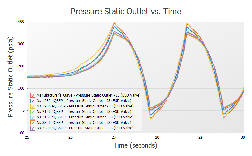
Figure 22: Static pressure at ESD Valve outlet for Case 2 using the manufacturer's curve and each of the four quadrant curve scenarios from 25 to 30 seconds
Step 7. Case 3 - Valve A Fails Open
A. Create Case Scenarios for Case 3
For Case 3, consider the scenario where flow is being transitioned to Tank B, like in Case 1. However, Valve A malfunctions and is stuck fully open so that Valve A and Valve B are fully open. In this case the elevation differences between Tank A and Tank B would cause Tank A to begin draining. To prevent Tank A from fully draining both the ESD valve and Valve B will be closed, and the pump will be intentionally tripped at the same time to bring the system to a safe stop so the Valve A malfunction can be investigated.
Make the following changes in the model:
-
In the Scenario Manager right-click on the Case 2 - Tank B to Tank A scenario and choose Clone With Children. Rename the scenario Case 3 - Valve A Fails.
-
Open the Properties window for Pump J2 and go to the Transient Tab. Under Initiation of Transient change the Time Absolute to 0 seconds so that the pump trip will begin at the beginning of the run.
-
Repeat step 2 for the ESD Valve, junction J3.
-
Open the Valve Properties window for Valve A, junction J5. This valve will need to be set to be open, and remain open throughout the transient.
-
On the Optional Tab, set the Special Condition to None.
-
On the Transient tab set the Transient Special Condition to Ignore Transient Data. This will allow us to keep the transient data entered, but prevent the transient from being used for this scenario.
B. Compare four quadrant curves to manufacturer's curve
Now that the scenario is fully defined, let's examine the results for the model using the manufacturer's curve.
ØRun the Case 3 - Valve A Fails scenario from the shortcut on the toolbar, or from the Analysis menu, and go to the Output window.
Once more we will see a warning indicating that the pump did experience reverse flow, which suggests a four quadrant curve should be used. Warnings will also be given for the transient static pressure, as were discussed for Case 2. Lastly, cautions will be given for reverse flow through junctions 5 and 7. These cautions occur since the loss factors through these junctions were entered assuming the losses were for forwards flow through the junctions, and may be inaccurate when reverse flow occurs. We will assume the difference is negligible in this case, though this should be verified for actual analysis.
In the Pump Summary at the top of the window, we can see that the pump operates at
In the Pipes section of the Output click the Pipes tab to view the steady state results for the pipes. Here we can see that pipes P4 through P6 experience reverse flow at the beginning of the run when both Valve A and Valve B are open, as is expected.
For this scenario the final steady state after the transient is when the pump has tripped and both Valve A and Valve B are closed. This is not meaningful for comparison as all flows will be zero, so the four quadrant pump head curves were simply compared to the initial steady state for the system, as is shown in Figure 23. The power curves can be seen in Figure 24.
As expected the 4QBEP and 4QSSOP curves for each value of specific speed are identical when operating at BEP, so we essentially only need to compare the manufacturer’s curve to 3 four quadrant curves. Since the BEP stays the same in all scenarios, the BEP curves are the same as in the other cases. Thus our conclusions are similar to the conclusions from Case 2.
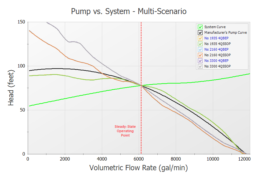
Figure 23: Pump vs. System Curve plot showing the manufacturer provided pump curve compared to pump curves from the
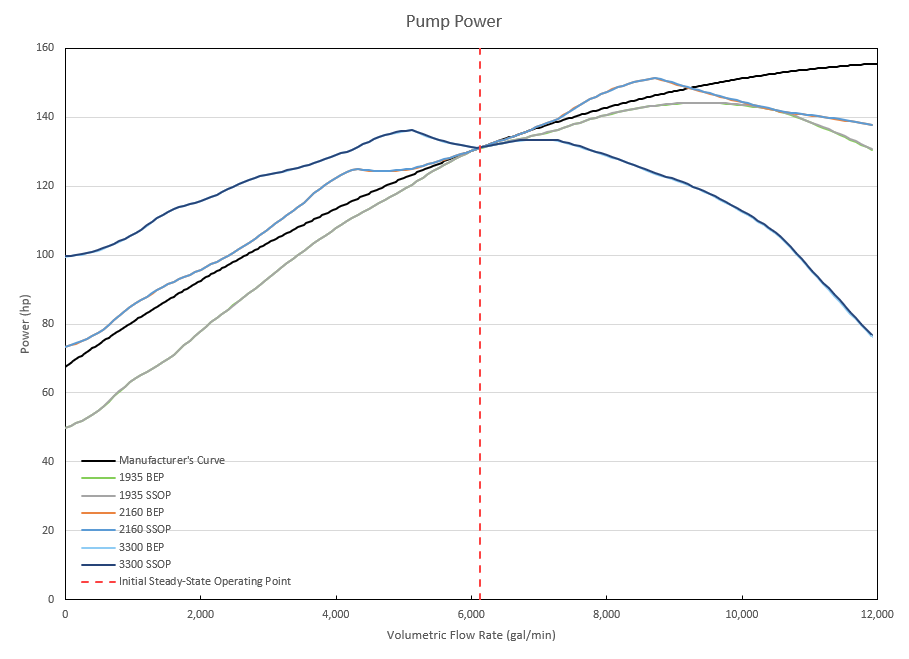
Figure 24: Pump Power Curve plot showing the manufacturer provided power curve compared to power curves from the
C. Examine transient results for Case 3
From Figure 25 and Figure 26 below it is clear that the four quadrant results diverge from the manufacturer's curve due to backwards flow beginning at the pump at about 3 seconds, and reverse rotation beginning at around 6 - 7 seconds, depending on the four quadrant curve. In Figure 27 we can see a comparison of the pressure results at the outlet of the ESD valve.
While the pump speed results show a significant difference between the scenarios, the velocity results at the pump and the pressure results at the outlet of the ESD valve show relatively minor differences between the four quadrant scenarios.
When the manufacturer’s curve results are compared to the four quadrant curves, we can see that the difference in reverse velocity is between
As with Case 2 it should be noted that the ESD valve does not represent the overall maximum/minimum pressures for this model, which instead occur at Valve B. Cavitation is predicted at Valve B, so the engineer would be required to address the low pressures at Valve B based on the requirements for this system.
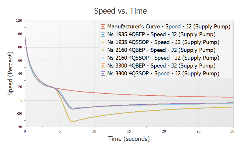
Figure 25: Pump speed vs time for Case 3 using the manufacturer's curve and each of the four quadrant curve scenarios
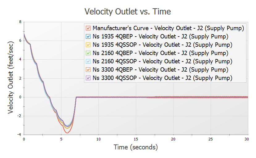
Figure 26: Velocity at pump outlet for Case 3 using the manufacturer's curve and each of the four quadrant curve scenarios
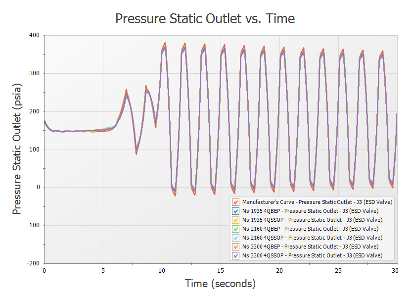
Figure 27: Static pressure at ESD Valve outlet for Case 3 using the manufacturer's curve (shown in black) and each of the four quadrant curve scenarios, which all overlap at the green curve
Conclusion
In this example three different pump trip scenarios were analyzed for a water transfer system in which there was potential for reverse flow and reverse rotation to occur at the pump. Four quadrant data was considered for use to accurately account for this potential reverse flow/rotation.
In situations such as with Case 1 the reverse flow was negligible, but the pump experienced negative head, requiring the engineer to consider four quadrant data. The manufacturer’s curve was considered most accurate up until 21 seconds into the run when negative head was calculated at the pump.
In Case 2 and Case 3 where the reverse flow and reverse rotation was significant in duration and magnitude, the four quadrant curves allowed for more accurate results to be found. By comparing the pump head and power curves to the curve data from the manufacturer four quadrant data sets could be selected for the analysis based on the initial steady state, and final steady state where applicable.
From the results above it is clear that the choice of four quadrant data set and dimensional reference point can have a large impact on transient results. Note that while a pump operating closer to BEP will typically be less impacted by the choice of dimensional reference point, this will not always be the case. Performing a sensitivity analysis such as what was described in this example will allow the engineer to determine the impact that using different four quadrant data sets and dimensional reference points will have on the results of the transient simulation.


