Pump Trip with Backflow - Four Quadrant Modeling (English Units)
Pump Trip with Backflow - Four Quadrant Modeling (Metric Units)
Summary
This example evaluates two parallel pumps tripping in a cooling tower. Various discharge valve closure times are analyzed to examine the impact on the system when the valves close quickly enough to prevent reverse rotation at the pump, and when the valves do not close completely before reverse rotation occurs in the pump.
Topics Covered
-
Specifying a pump curve and power curve in the Pump Properties window
-
Using one of the transient pump models which accounts for pump inertia
-
Using a four quadrant data set for the pump performance curve
-
Using four quadrant data to model reverse flow and reverse rotation in the pump
Required Knowledge
This example assumes the user has already worked through the Beginner: Valve Closure example, or has a level of knowledge consistent with that topic. You can also watch the AFT Impulse Quick Start Video (English Units) on the AFT website, as it covers the majority of the topics discussed in the Valve Closure example.
Model File
This example uses the following file, which is installed in the Examples folder as part of the AFT Impulse installation:
Step 1. Start AFT Impulse
From the Start Menu choose the AFT Impulse 9 folder and select AFT Impulse 9.
To ensure that your results are the same as those presented in this documentation, this example should be run using all default AFT Impulse settings, unless you are specifically instructed to do otherwise.
Step 2. Define the Fluid Properties Group
-
Open Analysis Setup from the toolbar or from the Analysis menu.
-
Open the Fluid panel then define the fluid:
-
Fluid Library = AFT Standard
-
Fluid = Water (liquid)
-
After selecting, click Add to Model
-
-
Temperature = 100 deg. F
-
Step 3. Define the Pipes and Junctions Group
At this point, the first two groups are completed in Analysis Setup. The next undefined group is the Pipes and Junctions group. To define this group, the model needs to be assembled with all pipes and junctions fully defined. Click OK to save and exit Analysis Setup then assemble the model as shown in the figure below.
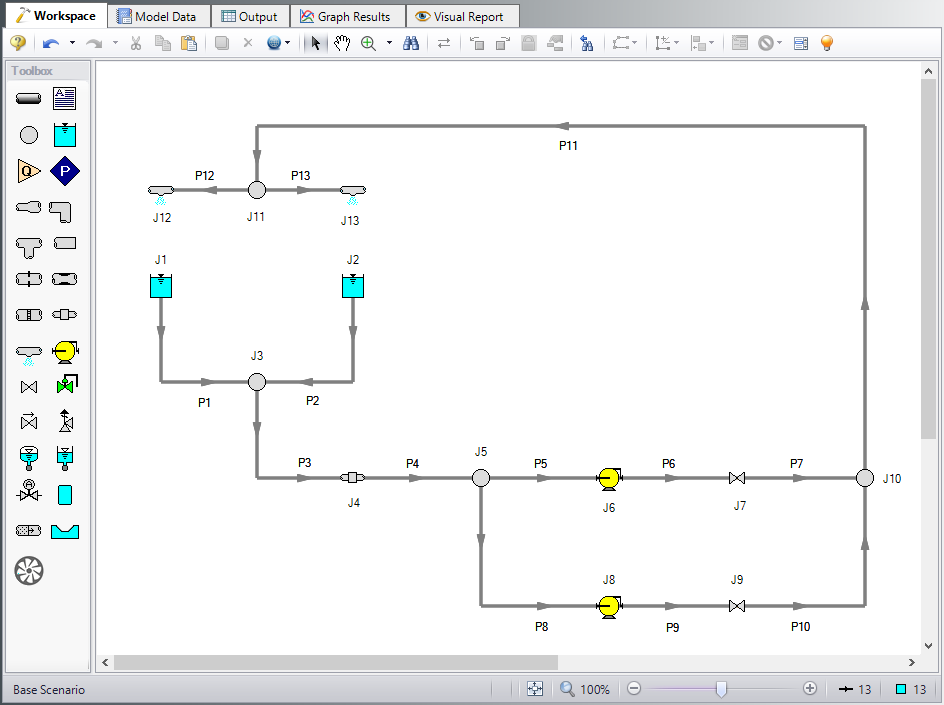
The system is in place but now we need to enter the input data for the pipes and junctions. Double-click each pipe and junction and enter the following data in the properties window.
Pipe Properties
-
Pipe Model tab
-
Name = Use table below
-
Pipe Material = Steel - ANSI
-
Size = Use table below
-
Type = Use table below
-
Friction Model Data Set = Standard
-
Length = Use table below
-
| Pipe | Name | Size | Type | Length (feet) |
|---|---|---|---|---|
| 1 | Pipe | 18 inch | STD | 40 |
| 2 | Pipe | 18 inch | STD | 40 |
| 3 | Main Supply | 30 inch | STD | 325 |
| 4 | Main Return | 30 inch | STD | 35 |
| 5 | CWP-1 Suction | 20 inch | STD (schedule 20) | 10 |
| 6 | CWP-1 Discharge | 20 inch | STD (schedule 20) | 10 |
| 7 | Pipe | 20 inch | STD (schedule 20) | 10 |
| 8 | CWP-2 Suction | 20 inch | STD (schedule 20) | 10 |
| 9 | CWP-2 Discharge | 20 inch | STD (schedule 20) | 10 |
| 10 | Pipe | 20 inch | STD (schedule 20) | 10 |
| 11 | CT Return | 30 inch | STD | 400 |
| 12 | Pipe | 20 inch | STD (schedule 20) | 40 |
| 13 | Pipe | 20 inch | STD (schedule 20) | 40 |
Junction Properties
-
Reservoir J1 & J2
-
J1 Name = CT #1 Basin
-
J2 Name = CT #2 Basin
-
Tank Model = Infinite Reservoir
-
Liquid Surface Elevation = 40 feet
-
Liquid Surface Pressure = 0 psig
-
Pipe Depth = 4 feet
-
-
Branch J3
-
Elevation = 35 feet
-
-
General Component J4
-
Name = Surface Condenser
-
Inlet Elevation = 0 feet
-
Loss Model = Resistance Curve
-
Enter Curve Data =
-
| Volumetric | Head |
|---|---|
| gal/min | feet |
| 0 | 0 |
| 20000 | 22 |
| 40000 | 88 |
-
Curve Fit Order = 2
-
Branch J5 and J10
-
Elevation = 0 feet
-
-
Pumps J6 and J8
-
J6 Name = CWP-1
-
J8 Name = CWP-2
-
Inlet Elevation = 0 feet
-
Pump Model tab
-
Pump Model = Centrifugal (Rotodynamic)
-
Performance Curve Used in Simulation = Standard Pump Curve
-
Rated Pump Speed = 1790 rpm
-
Enter Curve Data =
-
-
| Parameter | Volumetric | Head | Power |
|---|---|---|---|
| Units | gal/min | feet | hp |
| 1 | 0 | 112 | 105 |
| 2 | 2000 | 108 | 130 |
| 3 | 4000 | 104 | 160 |
| 4 | 6000 | 98 | 190 |
| 5 | 8000 | 90 | 210 |
| 6 | 10000 | 78 | 220 |
| 7 | 12000 | 60 | 210 |
-
Curve Fit Order = 2
-
Transient tab
-
Transient = Trip
-
Transient Special Condition = None
-
Initiation of Transient = Single Event
-
Event Type = Time Absolute
-
Condition = Greater Than or Equal To
-
Value = 0 seconds
-
Total Rotating Inertia = User Specified
-
Value = 140 lbm-ft2
-
Note: When reverse flow occurs at the pump, the Four Quadrant Model is recommended to obtain a better estimate for the head at reverse flow. To simplify the input, we will define the pump with the Standard Pump curve for now. We will come back later and compare these results to the Four Quadrant option.
-
Valves J7 & J9
-
J7 Name = Valve #1
-
J9 Name = Valve #2
-
Inlet Elevation = 0 feet
-
Loss Model tab
-
Valve Data Source = User Specified
-
Loss Model = Cv
-
Loss Source = Fixed Cv
-
Cv = 10000
-
-
Transient tab
-
Transient Special Condition = None
-
Initiation of Transient = Time
-
Transient Data = Absolute Values
-
-
| Time (seconds) | Cv |
|---|---|
| 0 | 10000 |
| 3 | 1000 |
| 5 | 0 |
| 15 | 0 |
-
Branch J11
-
Elevation = 50 feet
-
-
Spray Discharges J12 & J13
-
J12 Name = CT #1
-
J13 Name = CT #2
-
Elevation = 80 feet
-
Loss Model = Cd Spray (Discharge Coefficient)
-
Geometry = Spray Nozzle
-
Exit Properties = Pressure
-
Exit Pressure = 0 psig
-
Cd (Discharge Coefficient) = 0.6
-
Discharge Flow Area = 10 feet2
-
ØTurn on the Show Object Status from the View menu to verify if all data is entered. If so, the Pipes and Junctions group in Analysis Setup will have a check mark. If not, the uncompleted pipes or junctions will have their number shown in red. If this happens, go back to the uncompleted pipes or junctions and enter the missing data.
Step 4. Define the Pipe Sectioning and Output Group
ØOpen Analysis Setup and open the Sectioning panel. When the panel is first opened it will automatically search for the best option for one to five sections in the controlling pipe. The results will be displayed in the table at the top. Select the row to use one section in the controlling pipe.
Step 5. Define the Transient Control Group
ØOpen the Simulation Mode/Duration panel in the Transient Control group. Enter 15 seconds for the Stop Time.
To minimize run time and output file size, select to Save Output to File Every 10 Time Steps
Step 6. Run the Model
Click Run Model from the toolbar or from the Analysis menu. This will open the Solution Progress window. This window allows you to watch the progress of the Steady-State and Transient Solvers. When complete, click the Output button at the bottom of the Solution Progress window.
Step 7. Examine the Output
For this model several warnings and cautions will be shown in the output. A warning is given for both pumps stating that the pump experienced reverse flow and was using a Standard Pump Curve, meaning that the zero flow head value was used to predict head and power at reverse flow. Generally if the reverse flow is low in magnitude and duration using the zero flow head will be a good assumption and this error can be dismissed. For the purpose of this example we will compare the results from this scenario to the results using a four quadrant curve to examine the impact on the model.
There is also a caution given that the end of curve flow was exceeded in this model. Note that in this model we did not explicitly define the end of curve flow, so the last flowrate entered
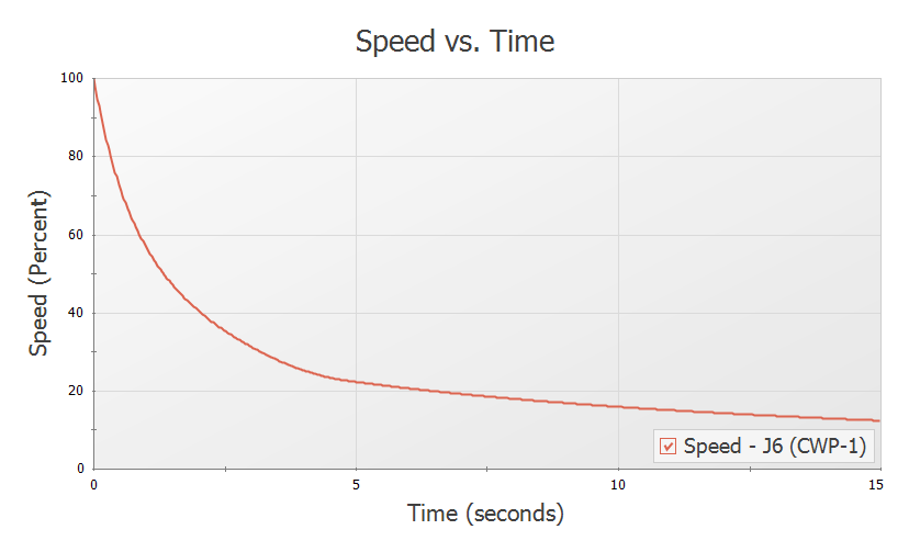
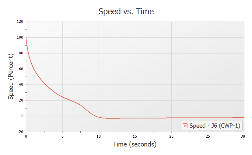
The speed of the two pumps should decay similarly. Figure 4 shows the speed decay for CWP-1. Here the pump speed decays quickly at first, then begins to slow after the discharge valve closes at about 5 seconds.
The transient pressure at the pump suction and valve #1 outlet is graphed in Figure 5, with the volumetric flow rate at these points on the secondary axis.
![]()
Figure 5: Transient pressures and volumetric flowrates at pump suction and discharge, and valve outlet
Step 8. Create Child Scenarios
To check the validity of our results when using the standard pump curve with an internal check valve to perform the pump trip with inertia, we should now go back and run the model with the pumps specified using four quadrant data for comparison. We will create three children scenarios, one for the current pump configuration using the Standard Pump Curve, and two using a Four Quadrant Data Set.
Note: Only one four quadrant data set is chosen for this example. In an actual four quadrant analysis it is recommended to compare multiple four quadrant data sets to ensure that the chosen data set is a good fit for the pump being modeled. See the Selecting a Pump Four Quadrant Curve example for more information.
To do this, click Create Child on the Scenario Manager on the Quick Access Panel. Name the child Standard Pump Curve. A new scenario will appear below the Base Scenario in the scenario tree. Select the Base Scenario, create another child, and call it Four Quadrant BEP. We will later clone this scenario to create our third child scenario.
The Standard Pump Curve scenario will use the pump settings that were already defined, so no changes will be needed for this scenario.
Step 9. Define the Four Quadrant BEP Scenario
Load the Four Quadrant BEP scenario by double-clicking the item in the Scenario Manager. Open the Pump Properties window for pump J6.
-
Performance Curve Used in Simulation = Four Quadrant Curve
-
Four Quadrant Curve = User Selected
-
Click Specify Model
-
Click Suggest a Data Set
-
AFT Impulse provides multiple pre-defined Four Quadrant Data sets which are characterized by specific speed. To choose a data set to use, we will first estimate the specific speed for the pump, which AFT Impulse will use to recommend a data set.
-
-
Flow/Head Source = Calculated from Standard Pump Curve
-
Calculated from Standard Pump Curve allows most of the data to automatically populate from the Pump Properties window. In this case, the pre-defined data is accurate for the pump.
-
-
Click Calculate
-
The Estimated Specific Speed in this case is
-
-
Click Select Suggested Data Set and Close
-
The Ns =
-
Note: It is always advised to select a Preferred data set close to the pump’s specific speed when possible. An Average data set may be selected if there are no close Preferred data sets, as was done here.
-
Dimensional Reference Point (DRP) = Best Efficiency Point
-
We will select the Steady State Operating Point option later for the third scenario.
-
-
Click OK on this window, then OK on the Pump Properties window to accept the changes.
-
Repeat the above steps for the other pump junction.
-
The required input for this scenario is now complete.
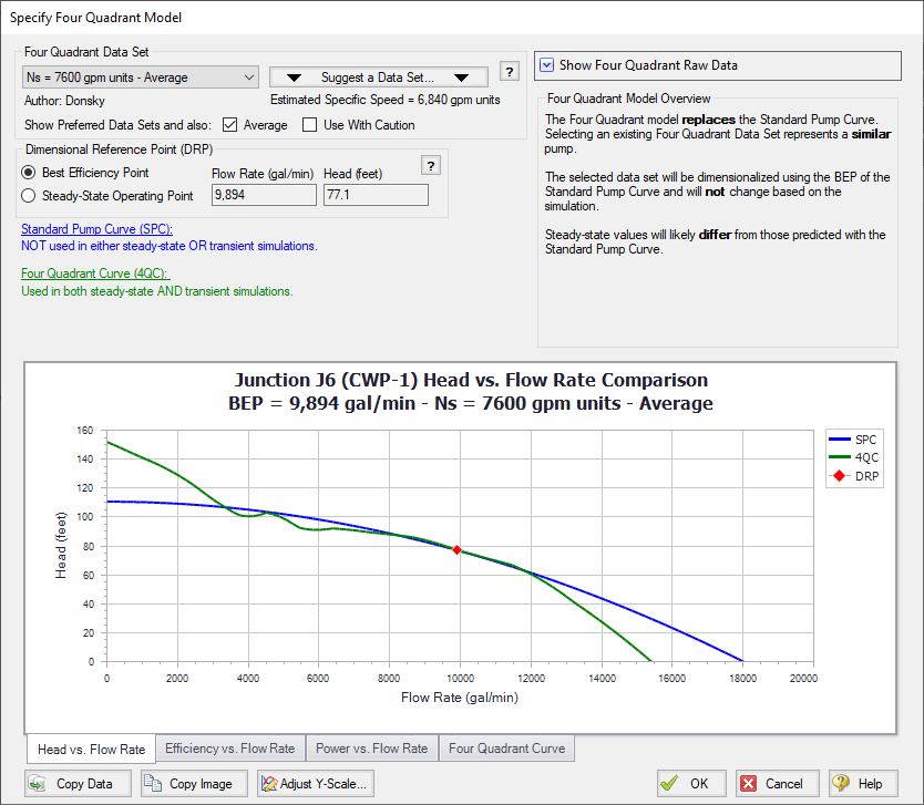
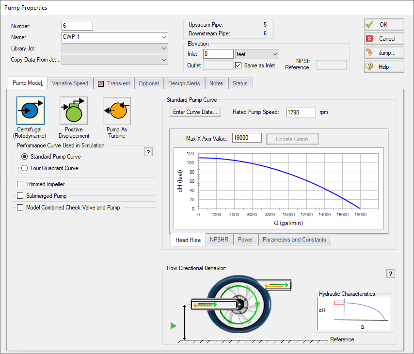
Figure 6: The Define Four Quadrant Model window can be used to select and view options for the dimensionalized four quadrant data set
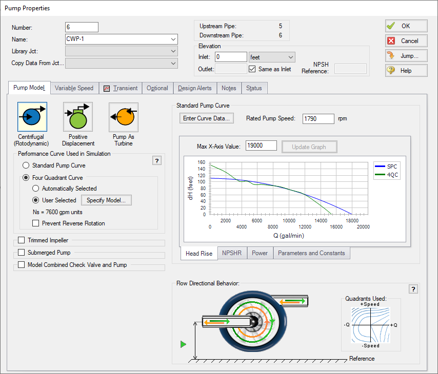
Figure 7: The Pump Model tab defined using the Four Quadrant Curve. Note that the Flow Directional Behavior section shows the pump behavior for both forwards and reverse flow and speed possibilities
Step 10. Define the Four Quadrant SSOP Scenario
Clone the Four Quadrant BEP scenario by right-clicking the scenario name in the Scenario Manager and choosing Clone Without Children. Name this cloned scenario Four Quadrant SSOP. For both pumps, open the Pump Properties window and click Specify Model under Four Quadrant Model. Change the Four Quadrant Curve Dimensional Reference Point to Steady-State Operating Point, then click OK on all open windows to accept the changes. The required input for this scenario is now complete.
Step 11. Run the Model and Examine the Output
Using the Scenario Manager load each of the four quadrant scenarios and run them. In comparing the transient results for the two four quadrant scenarios, there are no major visible differences. Figure 8 shows a multi-scenario graph with the pressures and volumetric flowrates for the Standard Pump Curve, Four Quadrant BEP and Four Quadrant SSOP scenarios. The two four quadrant scenarios produce results that are practically indistinguishable from the Standard Pump Curve results.
Comparison between the four quadrant graphs and standard pump curve graph reveals that the results are similar, though there is a visible difference of about
Now navigate to the Output window for each of the scenarios, then select the Pump Summary tab in the top third section. Notice that for the Four Quadrant SSOP and standard pump curve scenarios, the steady-state flow rate is
While the difference in steady state and transient results for the two dimensional points is minor in this model, it may become more pronounced in other cases. This choice of dimensional reference points can result in a trade-off between the accuracy of steady-state and transient data, especially if the pump operates further from BEP. Further details on this topic can be found in the Selecting a Pump Four Quadrant Curve example, as well as the main Help file for AFT Impulse.
On the Output window Warnings tab for each four quadrant scenario, information will be given on the four quadrant options that are defined in the pump, as well as listing topics which provide more background information on four quadrant data.
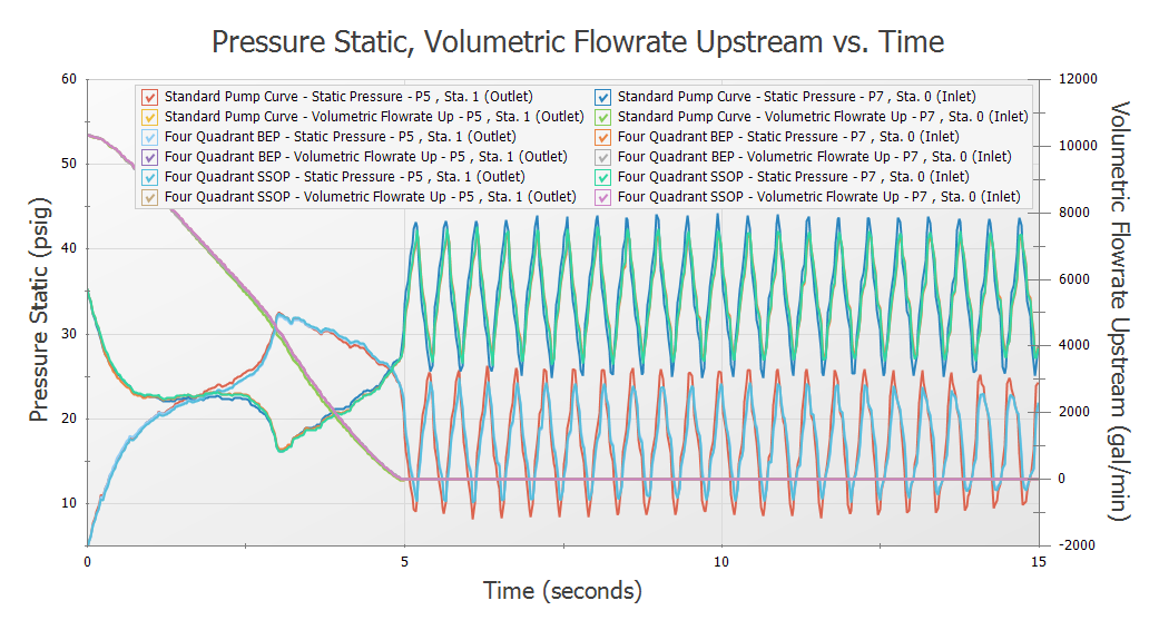
Figure 8: Comparison of Pressure and volumetric flow rate transients for the Standard Pump Curve, Four Quadrant BEP and Four Quadrant SSOP scenarios
Step 12. Adjust the Model
Consider the case where the valves at the discharge of the pumps cannot be closed in five seconds, but instead will close fully at twelve seconds. In this case the reverse flow at the pump will be significant due to the delay in the valve closure profile. We will need to use a four quadrant data set to analyze the effects of the possible reverse flow and reverse rotation in the pump, since the Standard Pump Curve does not have sufficient data. We will use the default selection to use the pump BEP as the dimensional reference point, though using the steady state operating point as the reference point would produce similar results.
In the Scenario Manager, select the Four Quadrant BEP scenario and create a child scenario named 12 Sec Valve Closure. The new child scenario should now be active. The pumps will already inherit the four quadrant model from the Four Quadrant BEP scenario, but the valves need adjustment. For both valves, open the Valve Properties window, then edit the Transient Data table found on the Transient tab to reflect the following closure profile.
| Time (seconds) | Cv |
|---|---|
| 0 | 10000 |
| 5 | 1000 |
| 12 | 0 |
| 30 | 0 |
Since the valve closure takes a longer time, it will be useful to extend the run time.
ØOpen Analysis Setup and navigate to the Simulation Mode/Duration panel and change the Stop Time to 30 seconds, then click OK.
Step 13. Run the Model
Click Run Model from the toolbar or from the Analysis menu. When complete, click the Graph Results button at the bottom of the Solution Progress window
Step 14. Examine the Output
The pressure and flow rate results are shown in Figure 9. Note that as expected, a significant amount of reverse flow occurs at the pump from about 6 to 12 seconds, requiring data beyond the standard data which is typically used for forward flow with forward rotation at the pump. The resulting transient results show that the maximum pressures at the valve outlet and the pump suction have been reduced.
The pump speed decay is shown in Figure 10. Note how the pump speed decreases at a faster rate than Figure 4. Additionally, at about 10 seconds the pump begins to experience reverse rotation. This means that from 5 seconds to 10 seconds, the pump will have forward rotation with reverse flow, then from 10-12 seconds, the pump will experience reverse flow with reverse rotation. Both of these situations can be accounted for using the additional information provided by the Four Quadrant Curve.
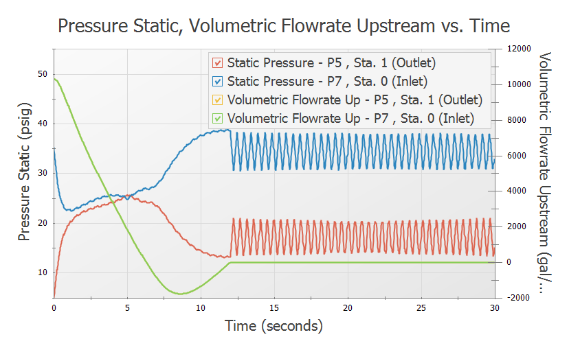
Figure 9: Predicted transient pump suction and discharge pressures and volumetric flowrates with a 12 second valve closure rate
Conclusion
For the valve closure of five seconds only a minimal amount of reverse flow was experienced at the pump. As a result, the standard pump curve was sufficient, since use of four quadrant data to accurately model this reverse flow had only a small impact on the results. Additionally, the choices of using the BEP or Steady State Operating Point to dimensionalize the four quadrant data were shown to be very similar in the transient, with minor differences in the steady state operating point. Changing the valve to close fully at twelve seconds resulted in significant reverse flow at the pump which required four quadrant data to be used. It was then found that increasing the valve closure time reduced pressures at the valve and pump.


