Relief Valve Modeling (English Units)
Relief Valve Modeling (Metric Units)
Summary
A system pumping crude oil over a long distance experiences a sudden valve closure. The pump is not able to stop before the valve is completely closed. A relief valve will be considered for surge mitigation.
Topics Covered
-
Modeling relief valve profiles during pressure surges
-
Examining the effect of valve rate limits on a system
-
Observing differences between relief valve profiles
Required Knowledge
This example assumes the user has already worked through the Beginner: Valve Closure example, or has a level of knowledge consistent with that topic. You can also watch the AFT Impulse Quick Start Video (English Units) on the AFT website, as it covers the majority of the topics discussed in the Valve Closure example.
Model Files
This example uses the following files, which are installed in the Examples folder as part of the AFT Impulse installation:
Step 1. Start AFT Impulse
From the Start Menu choose the AFT Impulse 9 folder and select AFT Impulse 9.
To ensure that your results are the same as those presented in this documentation, this example should be run using all default AFT Impulse settings, unless you are specifically instructed to do otherwise.
Step 2. Define the Fluid Properties Group
-
Open Analysis Setup from the toolbar or from the Analysis menu.
-
Open the Fluid panel then define the fluid:
-
Fluid Library = User Specified Fluid
-
Name = Crude Oil
-
Density = 0.85 S.G. water
-
Dynamic Viscosity = 4 centipose
-
Bulk Modulus = 200000 psia
-
Vapor Pressure = 10 psia
-
Step 3. Define the Pipes and Junctions Group
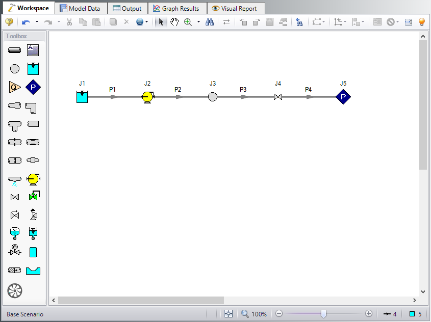
At this point, the first two groups are completed in Analysis Setup. The next undefined group is the Pipes and Junctions group. To define this group, the model needs to be assembled with all pipes and junctions fully defined. Click OK to save and exit Analysis Setup then assemble the model as shown in the figure below.
We will first evaluate the system without a relief valve to see if the maximum pressure of
The system is in place but now we need to enter the input data for the pipes and junctions. Double-click each pipe and junction and enter the following data in the properties window.
Pipe Properties
-
Pipe Model tab
-
Pipe Material = Steel - ANSI
-
Size = 24 inch
-
Type = STD (schedule 20)
-
Friction Model Data Set = Standard
-
Length = Use table below
-
| Pipe | Length (feet) |
|---|---|
| 1 | 20 |
| 2 | 10000 |
| 3 | 20 |
| 4 | 20 |
Junction Properties
To define the pump, a pre-built library will be used. We will need to first connect the library as follows
-
From the Library menu select Library Manager.
-
At the bottom, click Add Existing Library.
-
Browse to the Relief Valve Modeling.dat library file in the Impulse Examples folder and click OK. The library should now appear in the Library Browser under the name Relief Valve Modeling. Make sure the box is checked next to this library.
-
Click OK to exit the Library Manager.
Now proceed with defining the junctions.
-
J1 Reservoir
-
Tank Model = Infinite Reservoir
-
Liquid Surface Elevation = 10 feet
-
Liquid Surface Pressure = 10 atm
-
Pipe Depth = 10 feet
-
-
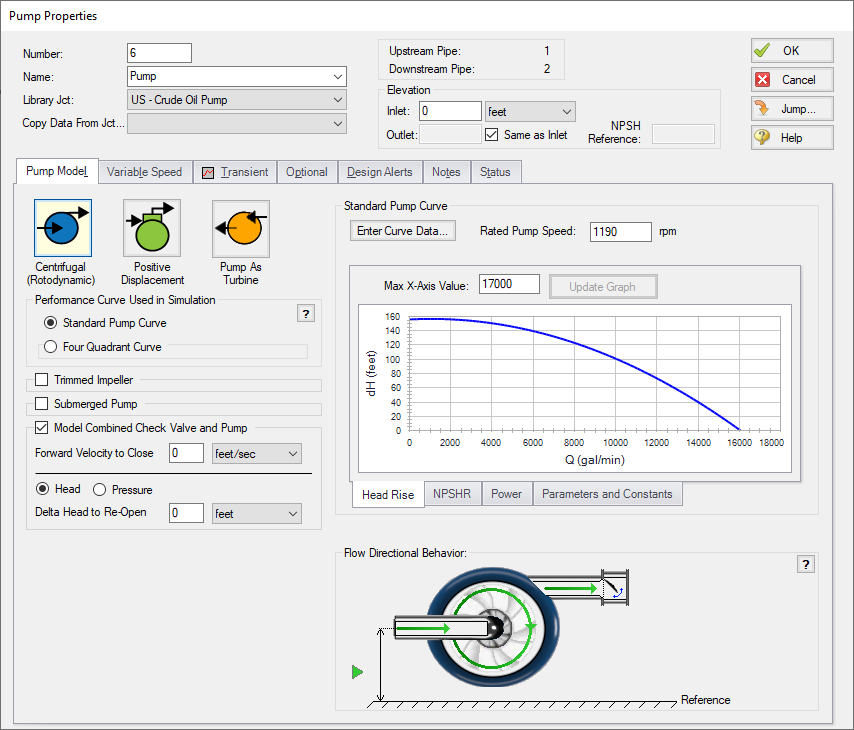
J2 Pump
-
Library Jct = US - Crude Oil Pump
-
Inlet Elevation = 0 feet
-
Note: The Model Combined Check Valve and Pump Option is used in this example to simplify the model. For higher accuracy it is generally recommended to model a check valve at the pump discharge using a Check Valve junction instead. See the Check Valve Modeling example for more information.
-
J3 Branch
-
Elevation = 0 feet
-
-
J4 Valve
-
Inlet Elevation = 0 feet
-
Loss Model tab
-
Valve Data Source = User Specified
-
Loss Model = Cv
-
Cv = 10000
-
-
Transient tab
-
Transient Special Condition = None
-
Initiation of Transient = Time
-
Transient Data = Absolute Values
-
-
| Time (seconds) | Cv |
|---|---|
| 0 | 10000 |
| 1 | 2000 |
| 2 | 0 |
| 30 | 0 |
-
J5 Assigned Pressure
-
Elevation = 0 feet
-
Pressure = 12 atm
-
Pressure Specification = Stagnation
-
ØTurn on the Show Object Status from the View menu to verify if all data is entered. If so, the Pipes and Junctions group in Analysis Setup will have a check mark. If not, the uncompleted pipes or junctions will have their number shown in red. If this happens, go back to the uncompleted pipes or junctions and enter the missing data.
Step 4. Define the Pipe Sectioning and Output Group
ØOpen Analysis Setup and open the Sectioning panel. When the panel is first opened it will automatically search for the best option for one to five sections in the controlling pipe. The results will be displayed in the table at the top. Select the row to use one section in the controlling pipe.
Step 5. Define the Transient Control Group
ØOpen the Simulation Mode/Duration panel in the Transient Control group. Enter 30 seconds for the Stop Time.
All groups should now be complete and the model is ready to run. If all groups in Analysis Setup have a green checkmark then Click OK and proceed. Otherwise, enter the missing information.
Step 6. Run the Model
Click Run Model from the toolbar or from the Analysis menu. This will open the Solution Progress window. This window allows you to watch the progress of the Steady-State and Transient Solvers. When complete, click the Output button at the bottom of the Solution Progress window.
Step 7. Examine the Output
The maximum pressure requirement for the line is
-
Go to the Workspace and select all of the pipes
-
Right-click the Workspace and select Generate Graph for Pipes > Pressure Static
-
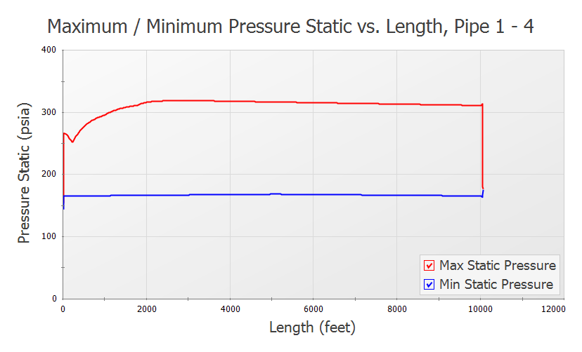
Click Add Graph to List and name it Static Pressure Profile
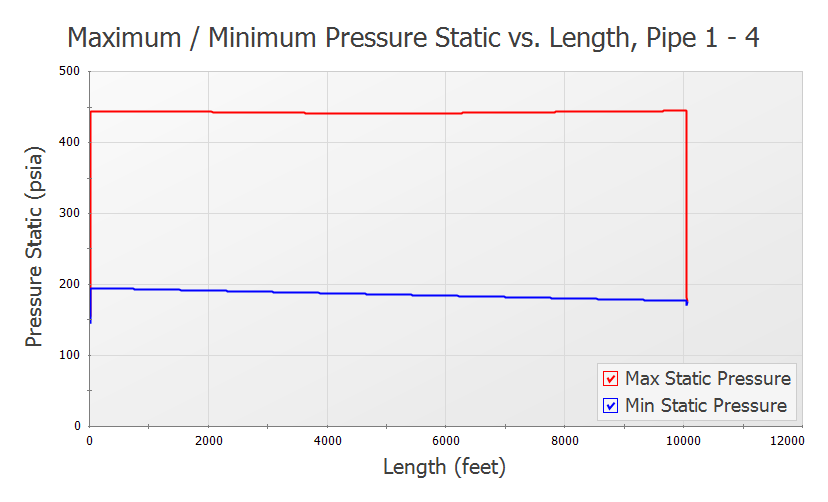
The maximum/minimum pressure profile graph can be seen in Figure 5. The pressure goes above the maximum pressure requirement for the majority of the line. To decrease the maximum pressure we will add a relief valve to the line near to the closing valve, which is the source of the pressure surge.
Step 8. Create Child Scenarios
We will create two scenarios to compare the model with and without a relief valve.
ØIn the Scenario Manager right-click the Base Scenario and click Create Child. Name the scenario No Relief Valve. Repeat this process to create a second scenario, Passive Relief Valve.
Now we will add the relief valve to the Passive Relief Valve scenario. Make sure the relief valve scenario is active in the Workspace by double-clicking the scenario name, then add a relief valve line as shown in Figure 6.
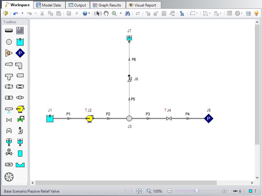
The crude oil will need to be contained in a closed vessel at the exit of the relief valve. For this example we will assume that the transient is fast, thus the pressure in the closed vessel will not change during the transient. The surge tank junction will be used to represent the closed, pressurized vessel. If the pressure in the closed vessel were to change significantly during the transient, then the surge tank would not be a good representation of this.
Define the additional junctions and pipes as follows.
Pipe Properties
-
Pipe Model tab
-
Pipe Material = Steel - ANSI
-
Size = 12 inch
-
Type = STD
-
Length = 20 feet
-
Junction Properties
-
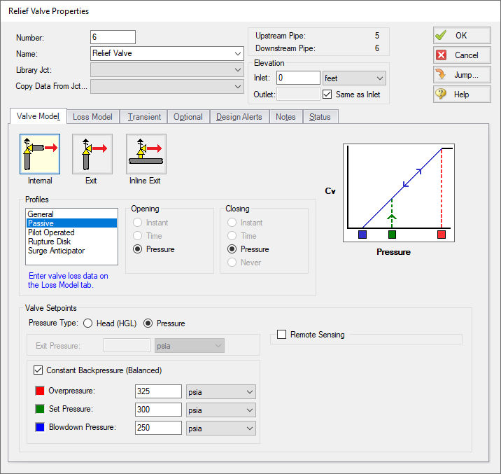
J6 Relief Valve
-
Inlet Elevation = 0 feet
-
Valve Model tab
-
Valve Model = Internal
-
Profiles = Passive
-
Pressure Type = Pressure
-
Constant Backpressure (Balanced) = Checked
-
Overpressure = 325 psia
-
Set Pressure = 300 psia
-
Blowdown Pressure = 250 psia
-
-
Loss Model tab
-
Loss Model = Cv (Variable)
-
Variable Data = Linear based on setpoints
-
Full Open Cv = 500
-
-
Note: The Ignore Relief Valve option on the Optional tab can be used to keep the relief valve closed. This is useful for running cases with no relief valve in the system, or where the relief valve fails to open without deleting the relief valve junction.
-
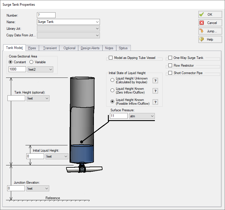
J7 Surge Tank
-
Cross-Sectional Area = Constant
-
Value = 1000 feet2
-
Initial State of Liquid Height = Liquid Height Known (Possible Inflow/Outflow)
-
Surface Pressure = 11 atm
-
Initial Liquid Height = 0 feet
-
Junction Elevation = 0 feet
-
Step 9. Define the Pipe Sectioning and Output Group
New pipes were added to the model, so the model needs to be sectioned again.
ØOpen Analysis Setup and open the Sectioning panel. When the panel is first opened it will automatically search for the best option for one to five sections in the controlling pipe. The results will be displayed in the table at the top. Select the row to use one section in the controlling pipe.
Step 10. Run the Model
Click Run Model from the toolbar or from the Analysis menu. When complete, click the Graph Results button at the bottom of the Solution Progress window.
Step 11. Examine the Output
Reload the Static Pressure Profile graph item by double-clicking the graph item in the Graph List Manager. The pressure profile should now appear as shown in Figure 9 below.
With the relief valve the maximum pressure reached in the pipeline is about
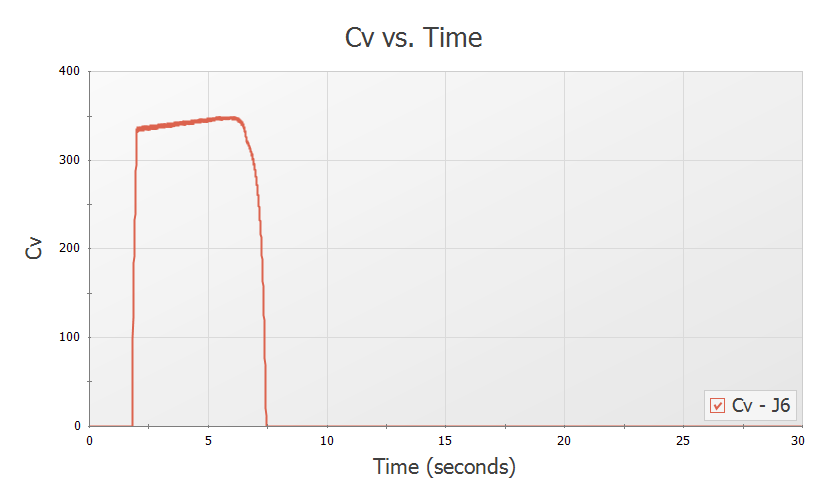
Now create a Transient Jct graph for the relief valve, and select Cv as the parameter to be graphed (Figure 10). Save this graph as Relief Valve Cv in the Graph List Manager.
Taking a closer look at the graph it can be seen that the valve opens over about 0.2 seconds, and closes over about
Step 12. Add Rate Limits to the Relief Valve
A relief valve's rate limit represents the rate at which the valve can open and close. If no rate limit is defined for the relief valve, it is possible for the valve to open/close nearly instantaneously. An instant opening for a relief valve is idealized, as the high pressures can be instantly alleviated in the pipeline once the valve setpoint is reached. Instant closure of the relief valve would represent the worst case scenario, as the rapid closure would produce the maximum pressure rise at the relief valve. In reality it is not physically possible for the relief valve to close in one time step. In addition, relief valve manufacturer's often design the valves to close slowly to avoid surge events that could occur due to a sudden closure. Adding rate limits allows for a more realistic representation of how fast the valve position can change over time.
Add rate limits to the relief valve as follows:
-
In the Workspace window, under Scenario Manager, create a new child scenario under the Passive Relief Valve scenario named With Rate Limits, and load it as the active scenario.
-
Open the properties window for Relief Valve J6.
-
On the Loss Model tab check the boxes next to both Apply Closing Limit and Apply Opening Limit (Figure 11)
-
Add a Max Closing Cv change of 150 and a Max Opening Cv change of 1500
-
Click OK
-
Run the Model, click on Graph Results
-
Open your saved graph Relief Valve Cv under Graph List Manager
-
In the Graph Parameters section, click the Multi-scenario button, then select the With Rate Limits and Passive Relief Valve scenarios.
-
Click Generate to create the graph as shown in Figure 12.
-
Repeat steps 7 and 8 above for the Static Pressure Profile graph, as shown in Figure 13.
In Figure 12 it can be seen that though the relief valve still opens in about 0.2 seconds, the relief valve now closes at a slower rate of about
From Figure 13 it can be seen that the slower opening speed results in a higher maximum pressure in the pipeline since the relief valve takes longer to fully open. The longer closing time practically eliminates surge waves caused by the closure of the relief valve, which causes a slightly lower minimum pressure along the pipeline.
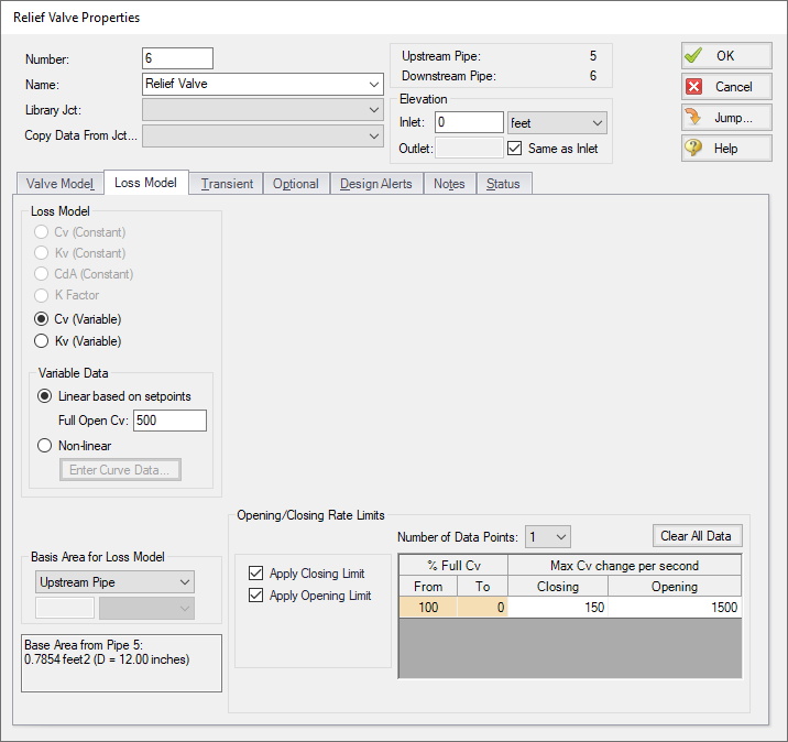
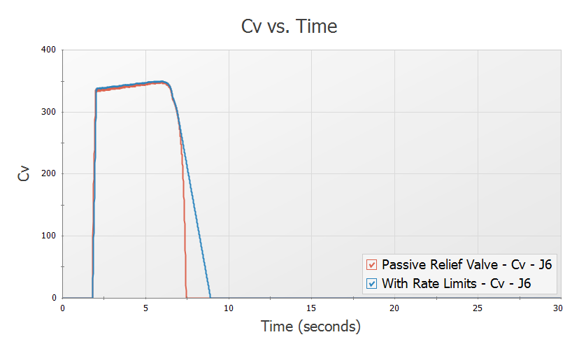
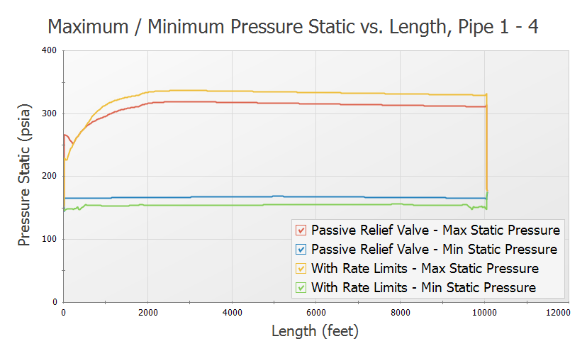
Figure 13: Comparison of maximum and minimum pressures along the pipeline when the passive relief valve is defined with and without rate limits
Step 13. Rupture Disk
We are now going to compare the passive valve above to a rupture disk relief valve. A rupture disk will burst open when the set pressure is met, and will remain open after that. The rupture disk will still relieve to a closed tank to keep the crude oil contained.
Update the model as follows:
-
In the Workspace window, under Scenario Manager, right click on the Passive Relief Valve scenario and choose Clone Without Children. Name the new scenario Rupture Disk.
-
Double click on the Relief Valve J6.
-
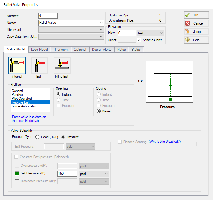
In the Profiles list select Rupture Disk (Figure 14)
-
Set Pressure (dP) = 150 psid
Note: The rupture disk will open on a pressure difference, unlike the passive relief valve which was defined using a fixed setpoint at which the relief valve would open. This is because the passive relief valve modeled previously had a mechanism to maintain a constant back-pressure on the valve, which is not used with the rupture disk. The pressure difference setpoint for the rupture disk was found by subtracting the outlet tank pressure from the desired opening pressure.
-
In the Loss Model tab, Cv (Constant) = 300
-
Click OK to close the window.
The scenario is now complete and ready to be run.
ØRun the Model and select Graph Results.
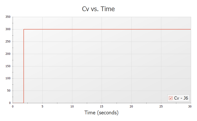
Load the Relief Valve Cv graph from the Graph List Manager, as is shown in Figure 15. Unlike the passive relief valve type, the rupture disk opens instantly, and remains open, as can be seen in the graph.
Next we want to compare the pressure results for each of the relief valve types.
-
Reload the Static Pressure Profile graph.
-
In the Graph Parameters area in the Quick Access Panel click the Multi-scenario dropdown and choose Select Scenarios
-
Select both the Rupture Disk and With Rate Limits scenarios, then click OK
-
Click Generate to incorporate the additional scenario (Figure 16)
The rupture disk generally maintains a lower maximum pressure in the pipeline, and overall reaches a lower minimum pressure. This makes sense considering that the rupture disk is allowed to open instantaneously (over one time step), thus the pressure in the pipeline is lowered faster for that scenario. In reality the rupture disk will not open instantaneously, but will still likely open faster than a passive relief valve type.
A lower minimum pressure occurs with the rupture disk because the rupture disk never closes.
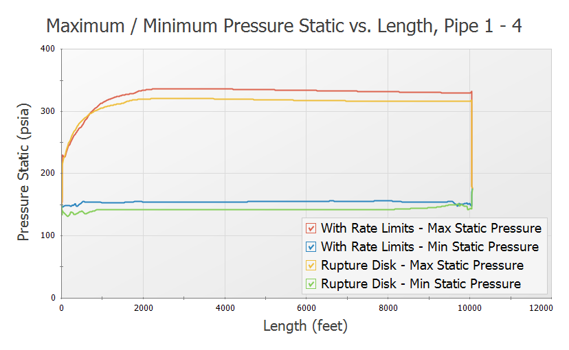
Figure 16: Comparison of maximum and minimum pressures with the passive and rupture disk relief valve types
Summary
Relief Valves provide pressure relief to systems during pressure surges. Impulse can model relief valves as an internal valve model, exit valve model, or inline exit valve model. An internal valve model connects two pipes acting as a gate providing relief from elsewhere in the system when necessary. An exit valve essentially models a spray nozzle at the end of a pipeline. An inline exit valve provides relief to the atmosphere along the length of some piping. These valve models can be profiled in a number of ways. In this example we worked with graphing results with a passive profile and rupture disk profile.


