Infinite Pipe Transient Theory
An infinite pipe is a representation of an interior pipe station - this is not the end of the pipe, but is identical to the same interior station in an equivalent system were the pipe is explicitly modeled. Therefore, all of the Method of Characteristics solution will apply to the infinite pipe boundary as well. However, by not explicitly modeling the entire pipe, there is some information we lose.
To determine the properties at the infinite boundary, we must know the properties of the adjacent stations from the previous time step. This is the case for any interior station. But this poses an immediate problem - there is only one "adjacent station" - we have removed the other by not modeling the pipe.
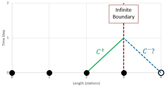
Figure 1: Downstream properties are required to calculate the negative characteristic
We can overcome this restriction by creating a "virtual" station one section past the end of the modeled pipe. Again, note that this virtual station represents a real interior pipe point, it is only "virtual" in the sense that no pipe is included in the model. With the virtual station, we then have stations adjacent to the boundary, and can proceed with the compatibility equations.
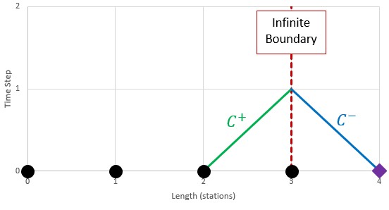
Figure 2: Create a "virtual" station to allow calculation of the negative characteristic
However, we have introduced a new problem. We need to know the pressure and flow at the virtual station to implement the compatibility equations for the subsequent time step. To proceed, we must estimate these values. This can be accomplished with the data we do know - adjoining stations and previous time steps. Without transient effects, we can make a very good approximation with a second order extrapolation.


This estimation requires data from the 3 adjoining stations, and 3 time steps previous.
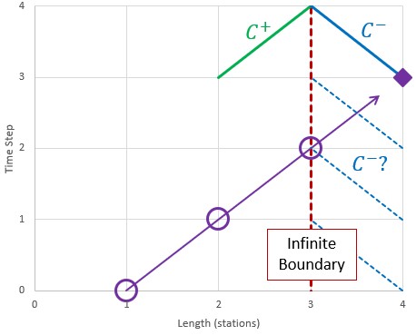
Figure 3: Estimate the properties at the virtual station with the 3 previous time steps and stations
This introduces yet another obstacle to overcome - if we require 3 stations and time steps for estimating the virtual station in the time step 3 (3 time steps after 0), we are not able to utilize the compatibility equations to calculate the properties at the boundary until time step 4. Fortunately, there is an easy solution.
The properties at the boundary can be considered constant until a transient from the system affects it. Any transient change requires 1 time step to travel 1 section. We can state that the properties at the boundary remain unchanged for the first 3 time steps if we keep the boundary at least 3 stations away from any potential transient perturbation. In other words, we need to require a minimum number of sections in the pipe. This minimum value is only two sections. This is because the initial transient time step (time step 1 in the diagram) can be considered the second fixed data point available to us - the first (time step 0) being the steady state initial conditions. The properties at station 1 cannot change until time step 2.
With a minimum of two sections, we can state that the pressure and flow at the boundary do in fact remain fixed for the first 3 time steps (4 including steady state).
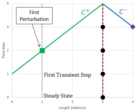
Figure 4: The estimation forces a certain minimum number of sections. Note that the properties cannot change at station 1 until time step 2 - one time step is required for any defined transient to impact the local solution.
See Wylie, et alWylie, E.B., V.L. Streeter & L. Suo, Fluid Transients in Systems, Prentice Hall, Englewood Hills, New Jersey, 1993., 1993, pp. 121-122 for more information.
Infinite Pipe Vapor Cavitation Theory
The Infinite Pipe junction is designed to only pass pressure waves out through the junction, and never to allow any reflections. If the junction drops to vapor pressure, a cavity would occur, which would cause reflections. Therefore, vapor cavities at these junctions are ignored and the pressure is allowed to fall below the vapor pressure. This maintains the function of the junction. If this occurs the model should be updated.
Related Topics
Related Examples


