Solution Method Panel

The Solution Method panel defines the calculation method and relevant parameters for the calculation (Figure 1). This panel is defined by default and typically should not be changed unless problems are encountered when running the model.

The Method Type can be set as Recommended or User Specified. The Recommended option (Length March With March Number Limits) is sufficient for most models. If desired the User Specified option can be selected to choose a different Method Type as are described below in the Solution Method Overview section below. Choosing User Specified also allows the march method increments to be changed.

A few other settings are defined by default for the user including the Length March Increment and Mach Number Increment settings. See the Marching Methods discussion below for more information on these parameters.

Lastly the "First Use Lumped Adiabatic..." option is available for all method types except the Lumped methods. This option solves the entire system with the Lumped Adiabatic method, and applies the results of that solution as a starting point to the marching method selected. This can help with convergence for some models. The results will be the same as using only the marching method. See the Lumped Methods section below for more information on Lumped Adiabatic.

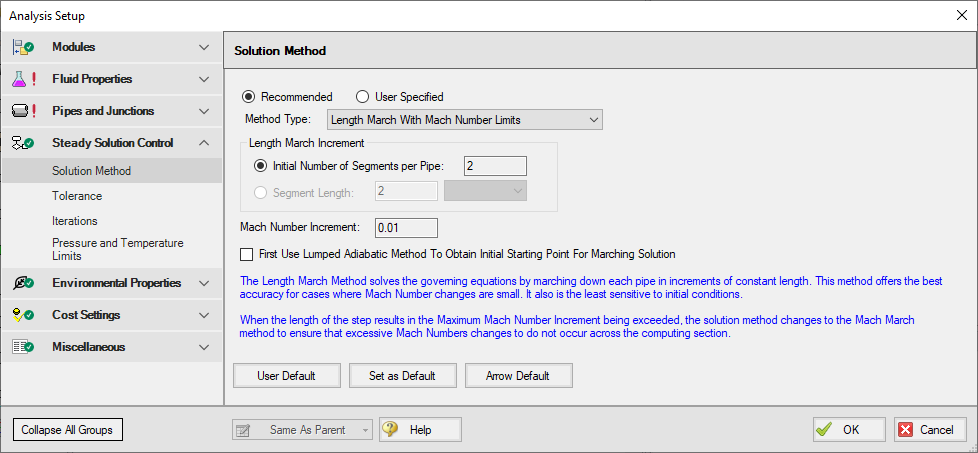
The Solution Method panel allows the user to define how AFT Arrow sets the segments in the pipe during the simulation

Figure 1: Default settings on the Solution Method panel

Solution Method Overview

AFT Arrow provides several solution methods for compressible pipe flow. Each method has certain advantages, and applicability to certain types of systems. While each option should theoretically come to a similar solution, there will be differences in the results between the methods. The magnitude of this difference depends heavily on the particular system being analyzed. All of the methods apply the same fundamental equations in differing ways.

Length March - All of the fundamental equations are applied at fixed length increments - axial points - down a pipe. This method provides good accuracy if changes in Mach Number are small. It is the least sensitive to initial conditions.
Length March With Mach Number Limits - This hybrid method starts with the Length March method, and dynamically switches to the Mach Number March method if the change in Mach Number between steps is large. This ensures excessive changes in Mach Number across computing sections are avoided.
Mach Number March - The fundamental equations are still applied at axial points down the pipe, but in this case the distance between the points is fixed by a Mach Number increment. This method is more accurate when there are large changes in Mach Number, often occurring when the Mach Number is high and when the flow is sonically choked.
Mach Number March With Length Limits - This hybrid method begins with the Mach Number March method, switching to Length March if the distance between axial points is too large. This helps ensure accuracy when the changes in Mach Number are small.
Lumped Adiabatic - This method ignores all heat transfer and elevation changes. For some applications these effects are minimal, and simplifying the calculations this way greatly reduces the required solution time and likelihood of convergence.
Lumped Isothermal - This method further simplifies the fundamental equations by assuming pipes are a fixed temperature throughout and again ignoring elevation.

Marching Methods

The marching methods provide the most accurate solutions. AFT Arrow "marches" down a pipe in the model, solving the fundamental equations along the way.

Dividing the pipe into smaller segments is important for compressible flow because the fluid properties change throughout the pipe. Each segment considers the flow properties constant and applies the fundamental equations. This represents a discretization of the continuously changing flow parameters - necessary for an iterative Solver such as AFT Arrow. This discretization introduces a certain amount of error into the solution, which is closely related to how many segments are present, as well as how much the flow properties change over a single segment.

When dividing the pipes into segments, axial points are created along the pipe, at the ends of every segment. The results at each axial point can be viewed in the output.

Length March - This method divides pipes into segments based on length. The segment length can be defined in two ways - either by dividing every pipe into a certain number of segments (Initial Number of Segments per Pipe setting), or dividing all pipes into equal-length segments (Segment Length setting). This method has the advantages that it is conceptually easier to understand and ensures some minimum number of segments in every pipe. Axial points are also often located at convenient locations. However, at high Mach Numbers, the large change in flow properties over a segment makes this method less accurate. For a detailed mathematical description of this method see Length March Method - Detailed Discussion.
Mach Number March - Unlike the Length March, Mach Number March determines the locations of the axial points dynamically based on the flow solution. There is no easy way to tell where the axial points will be without completing the solution. This method is superior when analyzing high Mach Number flows, as the flow properties tend to change dramatically over short distances. Effectively, this method adds axial points as necessary where the flow properties are changing rapidly. The disadvantage of this method is that the minimum number of sections cannot be enforced - if the Mach Number in a single pipe changes less than the increment specified, the entire pipe will be represented with a single segment. This is not necessarily inaccurate, but it is generally preferable to have more than one segment per pipe. For a detailed mathematical description of this method see Mach Number March Method - Detailed Discussion.

Hybrid Marching Methods

AFT Arrow offers hybrid marching methods to get the best of both marching methods in one solution. These methods dynamically switch from Length to Mach Number March or vice-versa during the solution.

This dynamic switch allows the user to ensure that a certain minimum number of segments is present in each pipe, and that the flow properties do not change significantly over the segment.

Length March With Mach Number Limits (AFT Arrow default) - The default solution method begins the march down the pipe with equal length segments. If the Mach Number over any certain segment is detected to increase more than the specified limit, the march continues over the rest of the pipe at equal Mach Number increments. It is often the case that flow velocity in a pipe is relatively low and constant in the first few segments of the pipe, but increases dramatically towards the exit. This method captures this behavior.
Mach Number March With Length Limits - Very similar to the default method, this hybrid method begins with a Mach Number march, but if it is detected that the length to the next axial point is too far due to relatively constant velocity, additional axial points are forced into the pipe via the length limit. This helps ensure all pipes have some minimum number of sections.

The figure below shows an example of a pipe solved with Length March With Mach Number Limits. During the solution, the solver determined that taking an additional 10 foot step from point 6 (60 feet) to point 7 (70 feet) would violate the Mach Number limit of 0.01. Therefore, the march was adjusted (starting at point 6) to increment in Mach Number steps of 0.01.

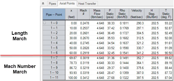
Figure 1: Length March dynamically switching to Mach Number March

Lumped Methods

For faster - but less accurate - computation, AFT Arrow offers two of the traditional lumped methods. These methods divide all pipes into 10 segments, but the method solves the entire pipe in a single computation. Certain assumptions simplify the fundamental equations allowing a much faster solution at the cost of accuracy.

Lumped Adiabatic - This method treats every pipe as adiabatic, disallowing heat transfer into or out of the pipe. If heat transfer is defined in the model, the definition is retained for convenience but is not applied during the solution. In addition, this model cannot accurately model body forces so therefore does not account for elevation changes or rotating systems. In many gas systems these assumptions are reasonable and the results from Lumped Adiabatic acceptable. For a detailed mathematical description of this method see Lumped Adiabatic Method - Detailed Discussion.
Lumped Isothermal - Similarly, this method treats all pipes as a constant temperature. Again, elevations are ignored. Note that heat transfer is applied to pipes (heat in or out) to meet the isothermal conditions. For a detailed mathematical description of this method see Lumped Isothermal Method - Detailed Discussion.
- Use Pipe Isothermal Temperatures When Available Instead of This Value - If Isothermal models have been defined for individual pipes, that temperature will be applied to that pipe instead of the global temperature defined in the Solution Method panel.

Comparing Marching Methods to Traditional Methods

There exist in industry practice a number of traditional methods and equations for calculating compressible flow in pipes.

A common equation is the Crane isothermal equation (see Crane, 1988, pp. 1-8). AFT Arrow and equations such as the Crane isothermal equation differ in several respects. First is that the Crane equation assumes isothermal flow, while AFT Arrow can model isothermal flow or other, more general, boundary conditions. Second is that the Crane equation solves the entire pipe as one segment. This can be called a lumped method. It is thus roughly analogous to using AFT Arrow with a single computing section per pipe. Third, the Crane equation assumes a constant diameter run, whereas AFT Arrow allows you to change diameters. Fourth, it is not apparent how to apply the Crane equation to multi-pipe systems, including pipe networks.

The Crane equation solves the governing mass and momentum equations by making some assumptions. AFT Arrow is solving the same equations, but is not making any assumptions. It marches down each pipe, taking into account physical property changes and non-linear acceleration effects as it progresses. Thus, AFT Arrow is in general much broader and more accurate than the Crane equation. When the pipe flow conditions are within the assumptions of the Crane equation, then the Crane equation and AFT Arrow should agree closely.

Other equations on page 1-8 of Crane, 1988, compare similarly to AFT Arrow. They are all lumped methods with certain assumptions about thermal conditions in the pipe and properties of the gas.

These traditional equations can be used successfully in many engineering applications. They all represent a subset of AFT Arrow’s marching methods, which solve the fundamental equations without limiting assumptions.