Mach Number March Method - Detailed Discussion
The Mach Number March Solution Method is described in detail below.
Modify Equation 2 by substituting Equations 3 and 5 and eliminating density,
|
|
(6) |

By definition of Mach number for a real gas
|
|
(7) |

and from basic calculus the following relationship holds:
|
|
(8) |

Differentiating Equation 7 (and using Equation 8) results in,
|
|
(9) |

Now, substitute Equation 7 and 9 into Equation 6 and eliminate the velocity
|
|
(10) |

Differentiating the equation of state, Equation 5 yields
|
|
(11) |

Replace velocity by Mach number by substituting Equation 9 into Equation 11 to obtain
|
|
(12) |

Eliminate pressure from Equation 10 using Equation 12 to obtain:
|
|
(13) |

From the definition of stagnation temperature
|
|
(14) |

Differentiating the preceding yields
|
|
(15) |

Replace static temperature in Equation 13 with stagnation by using Equation 14 and Equation 15 to obtain:

Collecting terms and simplifying yields:
|
|
(16) |

Rearrange Equation 16 to obtain
|
|
(17) |

Four useful parameters that simplify notation are:


|
|
(18) |

Using the four new parameters in Equation 18 simplifies to
|
|
(19) |

Integrating Equation 19 yields
|
|
(20) |

Equation 20 can be solved for x2:
|
|
(21) |

where the bars over certain parameters indicate that the average value over the computing section is used.
Equation 21 is the Mach Number March equation. The Mach Number March is a variable step size method. As shown in Equation 21, the distance is the parameter being calculated.
Modifications for Heat Transfer
In order to model heat transfer effects it is convenient in some cases to modify the previous equations.
The energy equation has the form:
|
|
(28) |

The definition of stagnation enthalpy is
|
|
(29) |

which, when substituted into Equation 28, yields:
|
|
(30) |

In most applications, the elevation term, gz, is very small and is neglected. This term will only become significant over pipes that have large elevation changes such as pipelines that go over mountains or down mineshafts, or in rapidly rotating systems.
With elevation neglected, it is not uncommon for engineers to conclude that adiabatic flow is isenthalpic (constant static enthalpy). It’s not. Rather, the stagnation enthalpy is constant in adiabatic flow.
Convective Heat Transfer
In pipe convective heat transfer, it is convenient to use the change in stagnation temperature rather than stagnation enthalpy by introducing the following approximation
|
|
(31) |

When heat transfer occurs, the effect of elevation change on the energy balance is small and is neglected. Substituting Equation 31 into Equation 30 yields
|
|
(32) |

The heat transfer due to convection is given by the following:
|
|
(33) |

where:
U = Overall heat transfer coefficient
Ph = Heated perimeter
The heated perimeter will frequently equal the wetted perimeter, which is the internal pipe circumference. It can change if part of the pipe is insulated (it will be less than the wetted perimeter) or there are fins on the pipe (it will be greater than the wetted perimeter).
Equating Equation 32 and 33 yields
|
|
(34) |

Rearranging Equation 34 yields:
|
|
(35) |

Integrating Equation 35 yields
|
|
(36) |

This relationship for stagnation temperature can be substituted into Equation 20 to obtain:
|
|
(37) |

In convective applications which use the Mach Number March method, the advantage of Equation 37 over Equation 21 is that the stagnation temperature change is proportional to the distance step dx (as shown in Equation 35), for which we are solving. Equation 37 couples the effects of friction and heat transfer, and provides more reliable convergence, especially in convection heating.
Constant Heat Flux
The constant heat flux boundary condition on a pipe results in a modified form of Equation 32
|
|
(38) |

The stagnation temperature change is thus:
|
|
(39) |

Integrating Equation 39 yields:
|
|
(40) |

Substituting this into Equation 20 yields:
|
|
(41) |

Example
Some examples are given here to clarify how the Mach Number March and Length March methods solve the governing equations.
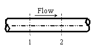
Figure 1: Marching equations are applied at successive computing sections along the pipe. Conditions at location 1 are known, and at location 2 are being solved using one of the marching equations.
Both of these methods are referred to as marching methods. What does this mean? Figure 1 shows a representation of a computing section in a pipe. In this example, all parameters at Location 1 are known, and it is desired to calculate conditions at location 2 which is always downstream of location 1.
Whether we are applying the Length March or the Mach Number March (Equation 21, 37 or 41), at location 1 we know these primary parameters:

Because we know the parameters above, we also know:

Let’s turn our attention to the Mach Number March method. Depending on the heat transfer model, AFT Arrow will solve either Equation 21, 37 or 41. The most general of these is Equation 21, so in the following discussion it will be referred to as the Mach Number March equation, with the understanding that Equation 21 encompasses Equations 37 and 41.
Similar to the Length March method, it is desired to solve for conditions at location 2 based on known conditions at location 1 (see Figure 2). However, here the length step itself is not known. In fact, as shown in Equation 21 it is the computing length (i.e., Δx) for which we are solving. What is the reason for trying to solve for Dx rather than just specifying it? This question will be answered shortly. Before that, let’s understand better what is happening when Equation 21 is applied.
The knowns at location 1 are the same as before, namely:

with the other derived knowns easily obtainable:

In the Mach Number March method, our step size is dictated by increments of Mach number. We thus take the Mach number at location 1 (M1) and add to it an increment. Since the maximum Mach number in the pipe systems modeled in AFT Arrow is 1, the step size should be far smaller. The default step size is 0.01. Using the default, we know the Mach number at location 2:


where ΔM is the Mach number increment. As before, we know the mass flow rate at location 2 (it's the same the same as location 1), and we also have similar heat transfer relationships as discussed in the Length March method example previously.
Specifically, if the pipe is adiabatic, we know the following at location 2:

or, if isothermal, the following is known at location 2:

and if the pipe has a convective or heat flux boundary condition,

However, in the convective and heat flux cases, we cannot definitely say what ho,2, is because the amount of stagnation enthalpy change depends on the length step, for which we are solving. This requires additional iteration.
Similar to the Length March method, the Mach Number March method requires significant iteration for each computing step. Again, known inlet conditions become the first location 1, and once location 2 is solved, it becomes location 1 and the marching continues to the end of the pipe.
Since we are solving for Δx, it is entirely possible that the distance step will extend beyond the pipe length. This will occur for any pipe that has an end-to-end Mach number change of less than ΔM. It will always occur for the final computing section of each pipe that does not reach choking. In such a case, the method reverts to the Length March method to compute conditions at the pipe exit.
It should be clearly understood that in the Mach Number March method, computing sections are not equidistant along a pipe. In fact, as the gas accelerates along the pipe, the Mach number increases more and more rapidly. This results in shorter and shorter computing section lengths as shown in the following application.
Example Application
Consider once again the model in Figure 2. All conditions are the same as in the previous Length March method application, except for the solution method. If we solve this model using the Mach Number March method, with a Mach number increment of 0.01, the results in Figure 3 are obtained.
There are several items to note about Figure 3. First, note how the Mach number increases down the length of the pipe. At the inlet, the Mach number is 0.2604 (this is not specified, but determined as part of the solution for flow rate). Each computing point increases the Mach number by DM , which is 0.01. This is what the Mach Number March method is, a method which marches in Mach number increments. With the step size dependent on the Mach number change, the number of calculation points in a pipe cannot be controlled. The 10 points shown in Figure 3 were chosen by AFT Arrow, not the user.
Second, note the x locations of computing points. These numbers are not whole numbers, and as the end of the pipe is approached the distance between each computing section and the previous one becomes smaller and smaller. This is a result of the gas acceleration. At higher Mach numbers this becomes even more pronounced.
Figure 4 shows how the Mach number increases along the pipe length. The curve's upward curvature shows the acceleration effect. Figure 5 shows the relative computing section distances.
Third, notice this adiabatic flow case has constant stagnation enthalpy, but not constant static enthalpy. This is similar to the Length March method.
Last, notice how the mass flow rate is (in this case) the same as the Length March method results shown in Figure 3 of Length March Method Example (4.884 lbm/sec). Since both methods solve the same governing equations, one would expect the results to be comparable. However, the two methods will not always agree. Each method has strengths and weaknesses, and results can differ somewhat when the flow conditions favor one of the methods.
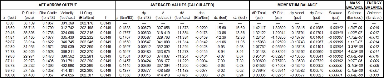
Is there any way to check that the results offer valid solutions of mass balance (Equation 1), momentum balance (Equation 2) and energy balance (Equation 30)? There is. An example is given in the Mach Number March Verification section below.
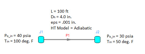
Figure 2: Model of an air system dropping from 40 to 30 psia
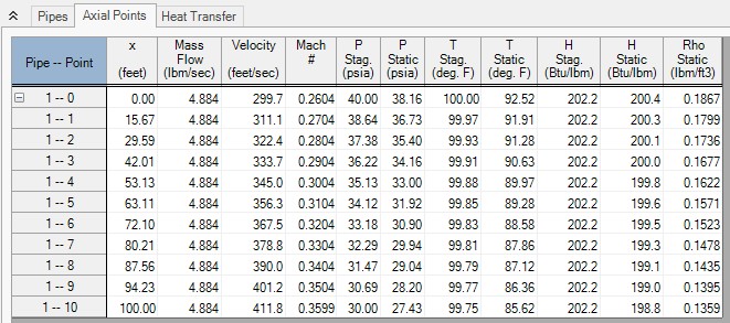
Figure 3: Axial Points (available in the Output window) for model in Figure 2 using Mach Number March method
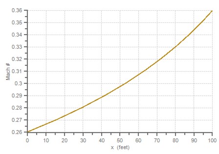
Figure 4: The Mach number increases with length in this plot of the Figure 3 results
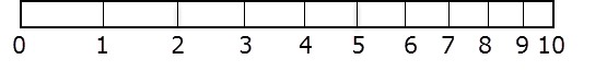
Figure 5: Relative pipe section locations for Figure 3 results. Notice how computing sections get closer as a result of gas acceleration as the end of the pipe is approached.
Mach Number March Method Verification
By changing the solution method for
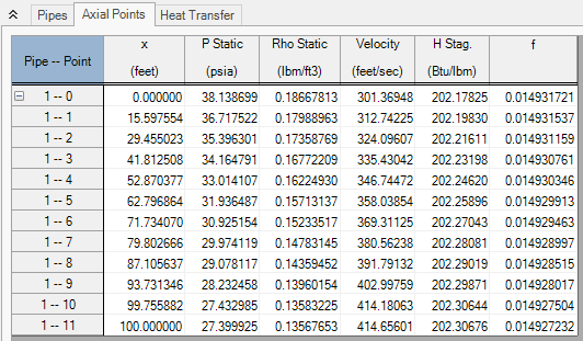
Figure 6: Axial Points for AFT Arrow model Verify_Governing_Equations.aro using the Mach Number March method
Table 1: Verification showing how AFT Arrow Mach Number March method predictions satisfy momentum, mass and energy balance equations. Taken from spreadsheet Verify_Governing_Equations_Mach.xls.