Length March Method - Detailed Discussion
The Length March Solution Method is described in detail below.
The stagnation pressure is given by the following:
|
|
(22) |

By differentiating Equation 22 the following is obtained:
|
|
(23) |

Now take Equation 23 and use it to replace the pressure term in Equation 10 to obtain:
|
|
(24) |

The first two terms on the right hand side of Equation 24 relate to the stagnation temperature (Equation 15) as follows:

Making this substitution, and also using Equation 14
|
|
(25) |

Integrating Equation 25 yields:
|
|
(26) |

And with algebra the Length March equation (Equation 27) is obtained:

|
|
(27) |

Example
Some examples are given here to clarify how the Mach Number March and Length March methods solve the governing equations.
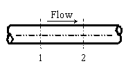
Figure 1: Marching equations are applied at successive computing sections along the pipe. Conditions at location 1 are known, and at location 2 are being solved using one of the marching equations.
Both of these methods are referred to as marching methods. What does this mean? Figure 1 shows a representation of a computing section in a pipe. In this example, all parameters at Location 1 are known, and it is desired to calculate conditions at location 2 which is always downstream of location 1.
Whether we are applying the Length March or the Mach Number March (Equation 21, 37 or 41), at location 1 we know these primary parameters:

Because we know the parameters above, we also know:

Let's consider the Length March method first because it is easier to grasp. Using the Length March equation, we know three things about location 2. First, we know the length step, as this is specified by the user. We also know that the mass flow rate is constant. Lastly, we know the heat transfer relationship specified by the user and can use this to determine a thermodynamic parameter.
For instance, if the pipe is modeled as adiabatic (q = 0), we can determine the stagnation enthalpy at location 2 using the following assumptions.
If there is no elevation change, then:

and according to the Energy equation:

Even if there is elevation change, we know what it is and can just add that into the energy equation and calculate ho,2 explicitly.
If the pipe is isothermal, then:

If there is convective heat transfer or known heat flux, we can solve Equation 36 or 40 for To,2 which allows us to calculate ho,2 and we are at the same point as with adiabatic.
Thus, if any boundary condition other than isothermal is specified, the following is known at location 2:

or, if isothermal, the following is known at location 2:

With one thermodynamic parameter known at location 2, we guess at the stagnation pressure solution to the Length March equation. This in effect gives us two known thermodynamic parameters, from which all the other parameters can be determined through state relationships. This requires significant iteration for each computing step.
For each pipe in the system, the marching is initiated at the pipe inlet where conditions are known. The known inlet conditions reflect the current solution state at the junction upstream of the pipe. This is location 1. Based on the user specified length step, the distance to location 2 is specified. The method just described is used to converge on the conditions at location 2. Once this convergence occurs, the previous location 2 becomes location 1 and a new location 2 is determined based on the step size. The marching continues to the end of the pipe.
If the user specifies an absolute length size (say 10 foot sections), a step may go past the end of the pipe. This will occur for any pipe that is shorter than 10 feet. For a longer pipe of say 12 feet, the first computing length will be 10 feet, while the second will be 2 feet.
It should be understood that in the Length March method, computing sections are equidistant along a pipe, aside from possible roundoff at the end.
Note: The process of converging on location 2 while marching down a pipe is referred to as a local iteration. It is local in that it does relate to what is happening in any other part of the model. AFT Arrow also has global iterations, which relates to iterations made on the entire system in trying to obtain complete system convergence. You can specify iteration limits for each type of convergence in the Iterations panel.
Consider the model in Figure 2. This model is of an air system modeled as a real gas using Redlich-Kwong and Generalized enthalpy. The Solution Method panel specifies Length March method with 10 segments per pipe. Results using the Length March method are shown in Figure 3.
There are several items worth noting in Figure 3.
-
Note that the second column shows the x location for each computation step. Point 1 will be identical to the pipe's inlet values. For this model, there were 10 steps along a 100 foot pipe, thus each step is equally 10 feet long.
-
Notice how the velocity and Mach number increase along the pipe length.
-
Notice how the static temperature drops. This is due to cooling of the gas as it expands with pressure drop.
-
Notice that the stagnation enthalpy is constant in accordance with adiabatic flow.
-
Notice how the static enthalpy drops along the pipe length. This shows that the flow is not isenthalpic.
-
Notice how the stagnation temperature drops slightly. This is a result of real gas effects. A perfect gas will have constant stagnation temperature and enthalpy in adiabatic flow with constant elevation.
These results can be viewed graphically by changing to the Graph Results window and selecting to graph a profile along a flow path.
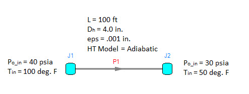
Figure 2: Model of an air system dropping from 40 to 30 psia
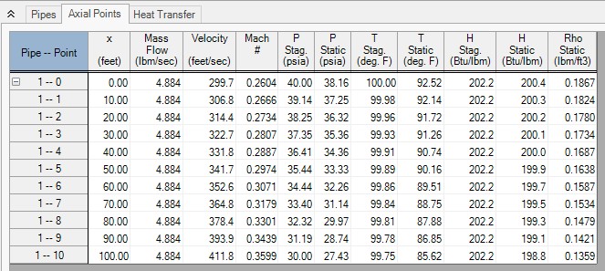
Figure 3: Axial Points (available in the Output window) for model in Figure 2 using Length March method
Length March Method Verification
The axial points shown Figure 3 can be used to verify that the fundamental equations are being solved accurately. Figure 4 shows the relevant verification parameters for a pipe carrying air from a tank at 40 psia and 100 deg. F to another tank at 30 psia. The pipe is vertical, 100 feet long, and 4 inches in diameter with a roughness of 0.001 inches, and is adiabatic. The high pressure tank is the top tank.

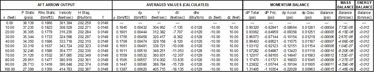
Figure 4: Axial Points for AFT Arrow model Verify_Governing_Equations.aro using the Length March method
The model,
The Figure 4 results were obtained using the Length March method with 10 pipe segments. The results can be copied to the clipboard and pasted into a spreadsheet as shown in Table 1. Once in the spreadsheet, additional calculations can be performed. Table 1 shows these calculations and a balance verification using all terms in the momentum equation (Equation 2), continuity equation (Equation 1), and energy equation (Equation 30). Along with the previous files, this spreadsheet is included upon request and is named Verify_Governing_Equations_Length.xls.
There are several terms in Table 1 that require clarification. Using coordinates as shown previously in Figures 1 of Fundamental Equations and Figure 1, density and velocity can be represented as follows:


Figure 5: AFT Arrow model solved in Figure 1 and verified in Table 1. Fluid is air. File is Verify_Governing_Equations.aro.
And using these terms, the four momentum equation terms from Table 1 are defined as:
| dP Total: |
|
|
| dP Fric. (Friction): |
|
|
| dP Accel (Acceleration): |
|
|
| dP Grav. (Gravity): |
|
(53) |


Table 1: Verification showing how AFT Arrow Length March method predictions satisfy momentum, mass and energy balance equations. Taken from spreadsheet Verify_Governing_Equations_Length.xls.
There is another term that is not relevant in this model and is thus not shown in Table 1. This term accounts for additional minor losses in the form of K factors, and is a modified form of the dP Acceleration term:
| dP Component: |
|

The four terms in Equations 53 in Table 1 are added together for each computing section. If the momentum equation is being satisfied, the four terms should sum to zero (or a very small number). They do, as shown in Table 1 in the column titled Balance (psi).
Note that AFT Arrow does not solve Equation 49. Rather, when using the Length March method, AFT Arrow solves Equation 27, which contains (more accurate) logarithmic terms. Equation 27 is a more complex form of the momentum equation. The arithmetically averaged terms in Equations 49 and Table 1 are approximations which show that the momentum equation is being satisfied.
Table 1 has another column titled Balance (lbm/sec) which shows that the continuity equation (Equation 1) is also satisfied. This is calculated in Table 1 as follows:

While not shown here, it was shown earlier in Figure 3 how AFT Arrow maintains constant stagnation enthalpy for adiabatic flow with zero elevation change. According to the energy equation (Equation 30), when the elevation changes, the stagnation enthalpy is not constant in adiabatic flow. The energy balance is calculated as follows:

In the Energy Balance column, Table 1 shows how this equation is satisfied. If heat transfer is applied, it is a simple matter to extend the spreadsheet behind Table 1 to verify that energy is balanced.
The individual terms in Equations 49 are also available for output in AFT Arrow. The contributions to pressure drop can be reviewed individually, and can also be used for further verification. Figure 6 shows the axial points again for Verify_Governing_Equations.aro, but now these pressure drop contributions are shown. The Output Control data configuration file used to obtain the Figure 6 format is Verify_Governing_Equations_2.dat.
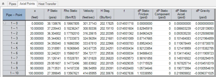
Figure 6: Axial Points for Verify_Governing_Equations.aro showing the individual pressure drop contributions
The Pipe Results table shows the total pressure drop contributions for each pipe when appropriate parameters are selected for display. See Figure 7.
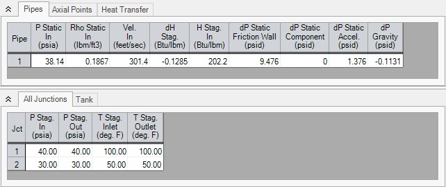
Figure 7: Pipe Results table shows total pressure drop contributions as defined in Equation 49


