Branch and Bound
Piping is almost always only available in Discrete sizes. Determining the best case selection of Discrete sizes requires a different approach than finding the best case Continuous sizes. One such method is Branch and Bound which is used for Discrete sizing on the basis of one of the Gradient Based Methods.
Branch and Bound divides the sizing problem into a collection of smaller sizing problems (branches). Solving these "sub-problems" gives information (bounds) about whether or not a given sub-problem is worth further investigation.
This method is well suited to problems with a relatively small number of variables (unique pipe sizes). For more than 10 variables, the Sequential Unconstrained method is advised. It is difficult to tell in advance how well any search method will work, and Branch and Bound is no different. It is possible, though unlikely, that the method can effectively reduce to a Brute Force Search. This makes it effective, but potentially very slow.
Example
There is a 50 foot pipe followed by a 100 foot pipe, and a 5 psi differential across the pipes. The piping is available in integer inside diameters between 3 and 17 inches, and the pipe walls thickness is always 10% of the inside diameter. Our goal is to minimize the weight of this system, while maintaining a flow of at least 2500 gal/min.
Even though there are only two independent pipe sizes to consider, with 15 possible pipe sizes, there are 225 possible permutations, more than we would like to test by brute force.
We start the process by finding the Continuous Optimum. For this example, this best case is (P1 = 8.75 in, P2 = 8.77 in, Weight = 2772 lbm). It is reasonable to assume that the Discrete Optimum will be near these sizes.
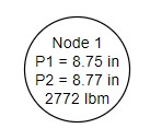
Figure 1: The first node showing the Continuous Optimum
From this first node, we want to divide the solution space on our first variable - the diameter of pipe 1. The pipe size cannot be 8.75 inches, it can only be a discrete size, in our case an integer value. Therefore, we branch the into two sub-problems with pipe 1 restricted to less than 8 or more than 9 inches (Figure 2). We have also established a bound on the problem - the solution will never have a feasible weight lower than 2772 lbm.
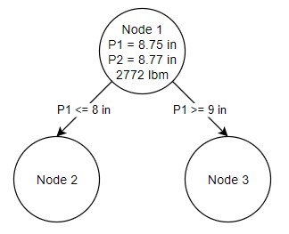
Figure 2: Two Sub problems are created from the Continuous Optimum in Node 1
It is important to note that these additional nodes represent continuous sub-problems. The pipe size is not forced to be discrete, it only has an additional requirement on it. The resulting pipe size will often be discrete because that continuous diameter is closest to the overall lowest feasible weight.
We can solve each of these independent problems with the same methods we used to solve the first node.
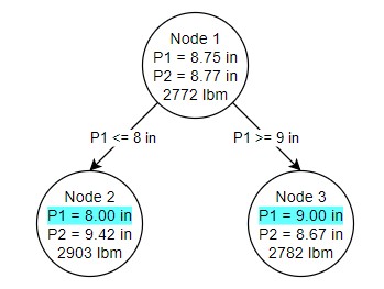
Figure 3: The conditions of Nodes 2 and 3 are shown, as well as the sizing arrived at in the two nodes
Due to the nature of this particular problem, the ideal pipe sizes for pipe 1 in both nodes 2 and 3 ended up as discrete sizes. This is not required or enforced by the method. Each of our nodes also has its own bound. This fact is used to determine the location of the next branch. Because node 3 has a better possible solution (2782 lbm) than node 2 (2903 lbm), we branch from node 3 (Figure 4). This time, however, we place a restriction on our second pipe's diameter.
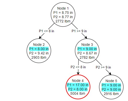
Figure 4: Node 4 produces an infeasible solution while Node 5 produces a feasible solution based on the branching criteria set from Node 3
Both of our branches from node 3 resulted in discrete size selections. However, node 4 was not able to result in a feasible solution. Infeasible nodes are valuable as there is no need to branch from them - placing further restrictions on a problem will never make it feasible. Node 5 on the other hand is both fully discrete and feasible. This is our first potential discrete solution. It is only a potential solution because node 2 has a lower bound - without branching from node 2, we do not know if a better discrete solution may exist under it, so branching from node 2 is exactly how we proceed (Figure 5).
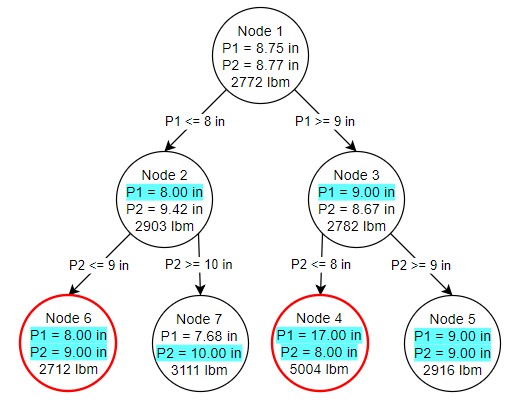
Figure 5: Branching occurs from Node 2 which produces one feasible (Node 7) and one infeasible (Node 6) solution
One of our nodes is infeasible, and despite the lower weight cannot be considered. Node 7, however, is feasible but not discrete, despite the requirements on diameter on both pipes. We could branch again from node 7, but there is no need - we have already found our ideal solution at node 5. We know this is the best possible discrete solution because the node 7 continuous solution has a higher minimum weight than node 5. No matter how we branch from node 7, we will never get a better solution than node 5.
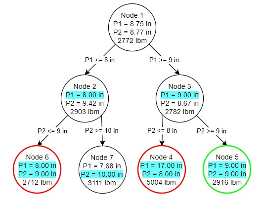
Figure 6: Results of the Branch and Bound method
Again, note that the results on node 5 are a continuous solution. It is only because of the requirements we have placed on the problem that the sizes have resulted in discrete sizes.
We have managed to find the best possible discrete solution by running 7 independent continuous sub-problems, instead of hydraulically solving hundreds of possible configurations. With more independent pipe sizes, the elimination of certain branches often becomes more common, further reducing the cases we need to check.


