Estimating the Gradient
Analytically determining the gradient becomes extremely difficult if not impossible for problems with many variables such as sizing a piping network. Instead, the gradient is estimated with a finite difference. This is a method for numerically estimating the gradient at a given point.
The test points created with a finite difference method each represent a hydraulic model that must be solved independently. If the model is complex, adding additional variables (unique pipe sizes) or required runs (from a central difference) can make the process take a significant amount of time.
Forward Difference
The Forward Difference estimates the gradient by finding the change in the function value by making a small change in the independent variable.
First, an initial result is found. We want to know the gradient at this point.
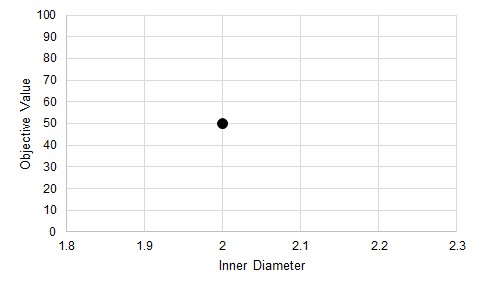
Figure 1: An initial test. It is desired to know the gradient at this point.
The independent variable is perturbed some small amount and a new result found. A line can be drawn through these two points - an estimate of the gradient at the initial point.
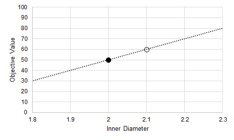
Figure 2: A perturbation. This allows the calculation of an average gradient as an approximation of the gradient at the initial point.
There are two important things to keep in mind:
-
This is an average gradient between the two points, but it is used as an estimate of the gradient at the initial point. It is not used to represent the behavior between the two points.
-
It is only an estimate. The result depends on the behavior of the Objective Function, and the selection of the test point.
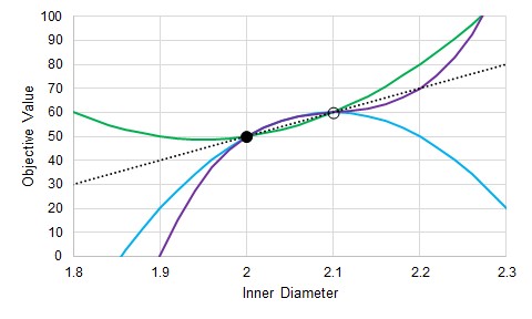
Figure 3: The actual gradient depends on the function. Many possible functions pass through two test points.
Central Difference
The central difference is a very similar process, with generally increased accuracy. We still want to know the gradient at our initial point (Figure 1), but instead of creating one test point, we create two, equidistant from the initial position. This effectively doubles the number of calculations required.
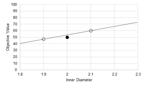
Figure 4: Central Difference estimate of gradient at the initial point
Relationship to Iterative Tolerance
It may seem that simply making the perturbation in the Inner Diameter smaller will increase the accuracy of the gradient and help reduce the issue indicated by Figure 3. If the Objective function was known explicitly, this would be a good assumption. However, in ANS, the results are not known explicitly. Instead, the solution is found via iteration. Iterative methods require some determination of convergence - namely, a tolerance on the solution. This means, by definition, that the results found are not the exact, analytical solution. Further, it is impossible to tell how the results may be biased away from the true solution.
When making test points, as before, there is some band of uncertainty in the Objective Value for the point related (but not necessarily equivalent) to the iterative tolerance.
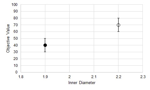
Figure 5: Uncertainty in the Objective Value due to iterative tolerance
We do not know where the "true" Objective Value lands on either of these bands, and we cannot state that the error is in the same direction or is of the same magnitude for both test points. This means that the gradient estimations have some variability as well.
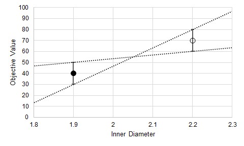
Figure 6: Uncertainty in the estimated gradient
In addition to the uncertainty indicated by Figure 3, there is also added uncertainty from the iterative tolerance.
It can be tempting to reduce the step size to increase gradient accuracy, but the iterative error will not be reduced. This can have dramatic results on the gradient.
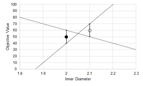
Figure 7: Substantially increased uncertainty in the estimated gradient from decreasing the step size
Now, due to the iterative tolerance, it is possible that the gradient is dramatically affected to the point where even the sign is uncertain.
Note: Making the step sizes too large impacts the gradient negatively in other ways. The critical thing to remember is that the step size should be small enough to capture the changing Objective, but not so small the iterative tolerance impacts the gradient quality.


