Cooling System - ANS (English Units)
Cooling System - ANS (Metric Units)
Summary
This example focuses on a closed loop cooling system that demonstrates some key features in using ANS to size a piping system. An existing model is used to investigate four potential sizing cases:
-
Size system for initial cost with a 10-year operating period
-
Size system for life cycle cost with a 10-year operating period
-
Size system for life cycle cost with an initial cost limit for a 10-year operating period
-
Size system for life cycle cost using a manufacturer's pump curve and with a 10-year operating period
The existing model was used to demonstrate AFT Fathom's capabilities for modeling closed-loop systems, pump curves, heat exchanger resistance curves, and fixed pressure drop control valves. This example will demonstrate how a system like the one built before can be seamlessly scaled up, meet design requirements, and minimize cost. For instance, the flow rate through the system will increase from
Note: This example can only be run if you have a license for the ANS module.
Topics Covered
-
Connecting and using existing engineering and cost libraries
-
Sizing for initial or life cycle cost
-
Using an initial cost limit with life cycle cost sizing
-
Sizing a pump and sizing piping for the chosen pump
-
Interpreting Cost Reports
Required Knowledge
This example assumes the user has already worked through the Walk-Through Examples section, and has a level of knowledge consistent with the topics covered there. If this is not the case, please review the Walk-Through Examples, beginning with the Beginner: Three Reservoir Model example. You can also watch the AFT Fathom Quick Start Video Tutorial Series on the AFT website, as it covers the majority of the topics discussed in the Three-Reservoir Model example.
In addition, it is assumed that the user has worked through the Beginner: Three-Reservoir Problem - ANS example, and is familiar with the basics of ANS analysis.
Model Files
This example uses the following files, which are installed in the Examples folder as part of the AFT Fathom installation:
-
Cooling System.dat - engineering library
-
Cooling System Costs.cst - cost library for Cooling System.dat
-
Steel - ANSI Pipe Costs.cst - cost library for Steel - ANSI pipes
Step 1. Start AFT Fathom
From the Start Menu choose the AFT Fathom 12 folder and select AFT Fathom 12.
To ensure that your results are the same as those presented in this documentation, this example should be run using all default AFT Fathom settings, unless you are specifically instructed to do otherwise.
Step 2. Open the model
Open the
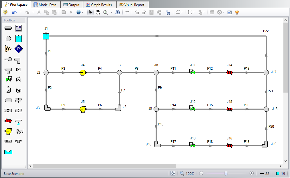
Although the model is fully defined, a few alterations are necessary for this example to scale up the system. First make sure that the Workspace looks like Figure 1 below:
Step 3. Define the Modules Panel
Open Analysis Setup from the toolbar or from the Analysis menu. Navigate to the Modules panel. For this example, check the box next to Activate ANS and select Network to enable the ANS module for use. A new group will appear in Analysis Setup titled Automatic Sizing. Click OK to save the changes and exit Analysis Setup. A new Primary Window tab will appear between Workspace and Model Data titled Sizing. Open the Analysis menu to see the new option called Automatic Sizing. From here you can quickly toggle between Not Used mode (normal AFT Fathom) and Network (ANS mode).
Step 4. Define the Fluid Properties Group
-
Open Analysis Setup from the toolbar or from the Analysis menu.
-
Open the Fluid panel then define the fluid:
-
Fluid Library = AFT Standard
-
Fluid = Water (liquid)
-
After selecting, click Add to Model
-
-
Temperature = 70 deg. F
-
Step 5. Define the Pipes and Junctions Group
As an initial guess to the scaled up system, we will change all pipe sizes to 36 inch. This should satisfy all Design Requirements and be a feasible solution, therefore it should be an acceptable initial guess for the system. Similar the junctions will be updated for the scaled up system.
Pipe Properties
Make the following changes to all pipes
-
Pipe Model tab
-
Size = 36 inch
-
Type = STD
-
Junction Properties
Make the following changes to these junctions.
-
J1 Reservoir
-
Liquid Surface Elevation = 30 feet
-
Liquid Surface Pressure = 0 psig
-
Pipe Elevation = 0 feet
-
-
J11 & J12 Control Valves
-
Valve Type = Flow Control (FCV)
-
Control Setpoint = Volumetric Flow Rate
-
Flow Setpoint = 2000 gal/min
-
Always Control (Never Fail) = Unchecked
-
-
J13 Control Valve
-
Valve Type = Constant Pressure Drop (PDCV)
-
Control Setpoint = Pressure Loss
-
Pressure Drop = 5 psid
-
-
J14-J16 Heat Exchangers
-
Enter Curve Data =
-
| Volumetric | Pressure |
|---|---|
| gal/min | psid |
| 0 | 0 |
| 2000 | 50 |
| 4000 | 200 |
Step 6. Overview of Sizing Systems with Pumps
A centrifugal pump can be modeled with either the Pump Curve or Sizing Analysis Type. Generally if a specific pump has been identified the Pump Curve type would be chosen, whereas the Sizing option is useful during the selection stage in order to identify the pumping requirements for the system. In some cases even though the specific pump has not been chosen several candidate pumps are available. For this third case it would be best to model each candidate pump as a pump curve using separate scenarios for each pump.
Sizing a Pump
The pumps in our cooling water case are being sized, so the Sizing Analysis Type was used with assigned flows of
As already stated, when a pump is modeled as an assigned flow, it is not a specific pump from a specific manufacturer. Thus, the costs for the pump can only be approximated. To a first approximation, it should be possible to estimate the non-recurring cost (i.e., material and installation cost) for the pump as a function of power requirements. For instance, a typical one horsepower pump may cost $2000, and a ten horsepower may cost $4000. Other typical costs for different power requirements can be approximated. The actual cost for the pump will, of course, highly depend on the application. Pumps for special applications such as corrosive fluids or high temperatures may have different cost structures, but a reasonable approximation of cost for various power usage levels should be possible. These costs are entered into a cost library, and are accessed by the solver. As ANS evaluates different combinations of pipe sizes, each combination will require a certain power from the pump. With a cost assigned to this power, ANS can obtain a cost to enter into the objective function that it minimizes. Later in this example, we will look at the costs for the pumps.
In addition to non-recurring costs, recurring costs can also be estimated. Specifically, the cost of the power used by the pump over a period of time can be determined. All ANS needs is an overall pump efficiency to determine an actual power from the ideal power. Again, since we do not have a specific pump selected yet, the efficiency can only be approximated. ANS calls this the Nominal Efficiency. In addition, users can provide a Nominal NPSHR.
One may ask how important it is to choose appropriate values at this level. It depends. If the model only sizes for non-recurring costs, then the nominal efficiency will affect the actual power requirement of the pump, and hence the cost obtained from the cost library. If the cost of the pump is large compared to the cost of the piping, the specified nominal efficiency will likely play a significant role in the system selection.
In addition, for models that include energy costs in the objective, the energy cost may be a minor or major portion of the overall system cost. If it is a major portion, the results of the sizing will likely be very sensitive to the specified nominal efficiency.
Therefore, it is recognized that at this first cut phase the values for nominal efficiency and nominal NPSHR are imprecise and users may need to go through a few iterations to arrive at satisfactory results.
Modeling Pumps with a Pump Curve
When one is modeling a pump curve, accurate NPSHR and efficiency (or power) requirements can be specified for the pump. The cost data for that pump can also be accurately specified. During the automated sizing run the impact of the pump on the system sizing will be in the area of energy costs and in the requirement to satisfy the pump's design requirements.
First, let's discuss the issue of recurring cost. The non-recurring costs for the pump will be fixed, and will therefore not impact the sizing process. However, energy costs will vary with the power required for the pump. Thus including energy cost in the sizing will influence the pipe size selection.
Second, the specific pump has certain design requirements. For example, the sized network will be of no value if the NPSHR is violated. Thus, the pipes have to be selected by ANS in such a way as to satisfy all pump design requirements.
Since a specific pump is not input for our cooling water model (yet), no specific pump selection can happen at this point. It may frequently be the case that, based on the results of modeling the pump as an assigned flow pump, several candidate pumps may exist. The best approach is to create a scenario for each of these pumps, and rerun the sizing for each candidate pump. This will yield an ideal candidate pipe system for each candidate pump, from which an educated choice can be made for the system design. All else being equal, the selection would be the candidate pipe system that offers the lowest cost. When approached in this manner, one is selecting the pump and the piping system as an entire system, which offers improved matching of the pump to the system, and also offers significant opportunity for cost reduction.
Summarizing the Pump Selection Process
Based on the preceding discussion, we can outline a process for selecting a pump that offers a matched pump and piping system at the lowest possible cost. This discussion is an extension of the discussion in the Fathom Help file regarding sizing pumps and pipes concurrently. Here, we will augment that discussion with the considerations that are relevant to sizing.
-
Phase 1: Size the pump
-
Model the pump (or pumps) as assigned flow pumps using the Sizing Analysis Type. If flow control valves exist, select the one that offers the lowest pressure drop margin (as discussed in the AFT Fathom Help file), and set that one to a pressure drop control valve at the minimum required pressure drop.
-
The largest uncertainty at this point is the cost of the pumps. Based on actual pump cost data, specify the approximate cost of pumps of different power levels for different flow rates. This is entered into a cost library.
-
Along with the design flow rate, specify a nominal efficiency that is consistent with the application and your experience. If you are unsure, take a guess and, after completing Phase 1, return to this step and improve your guess.
-
If you have a reasonable idea of what the NPSHR will be, specify that in the nominal NPSHR. If you are unsure, ignore nominal NPSHR and proceed. After completing Phase 1, check the NPSHA and make sure that pumps are available at the head requirements obtained from the ANS results that have sufficient NPSHR margin.
-
Determine whether the design goal is to minimize initial cost or life cycle cost, and select the appropriate objective in the Sizing Objective panel.
-
Run the model and review the results. Take note of the relative cost difference between the piping and the pump(s). If the pump costs are a significant percentage, then continued iteration on Phase 1 will likely be worthwhile. Continued iteration would involve obtaining more precise cost information for pump(s) at the flow, head and power usage levels obtained from the Phase 1 results. It would also involve obtaining more precise information on nominal efficiency and nominal NPSHR.
-
-
Phase 2: Select a pump
-
Phase 1 worked with approximate cost and engineering data for your pump. With that information ANS sized the network for an optimal pipe and pump system combination. At this point, that optimal system should be viewed as preliminary. Based on the pump operating point from Phase 1, identify some candidate pumps that match the requirements.
-
Change any flow control valves set to pressure drop control valves (as specified in Phase 1a) back to flow control valves.
-
Identify the operational requirements for the flow control valves, such as minimum pressure drop, and enter those as Control Valve Design Requirements.
-
For each candidate pump, create a child scenario. Each child scenario should be created below the scenario that has the flow control valves as discussed in Phase 2a and 2b.
-
Enter the pump head, NPSHR and efficiency (or power) curve. Enter the actual pump cost as well into a cost library.
-
Run each scenario. All else being equal, the scenario with lowest cost will be the preferred design. The pipe sizes obtained from this final solution may differ slightly from those obtained Phase 1. If there are significant pipe size differences between Phase 1 and Phase 2, it may indicate that the actual pump was not matched very well to the Phase 1 requirements. It could also mean that there was an error somewhere in the process.
-
In Phase 2f, it may not be true that all else is equal. For example, even if one design offers lower cost, you may prefer a higher cost system because your experience suggests the pump is more reliable. On another note, if it is possible to quantify the cost reliability, this can be included in the cost of the junction and the automated sizing process.
-
For this example, we will be completing the pump selection process above considering the objective of minimizing initial cost, then minimizing life cycle cost.
Step 7. Configure Sizing Settings
Load the Base Scenario. The hydraulic model is already defined for a regular Fathom run, but we need to complete the sizing settings before running the analysis. Navigate to the Sizing window by clicking the Sizing tab at the top.
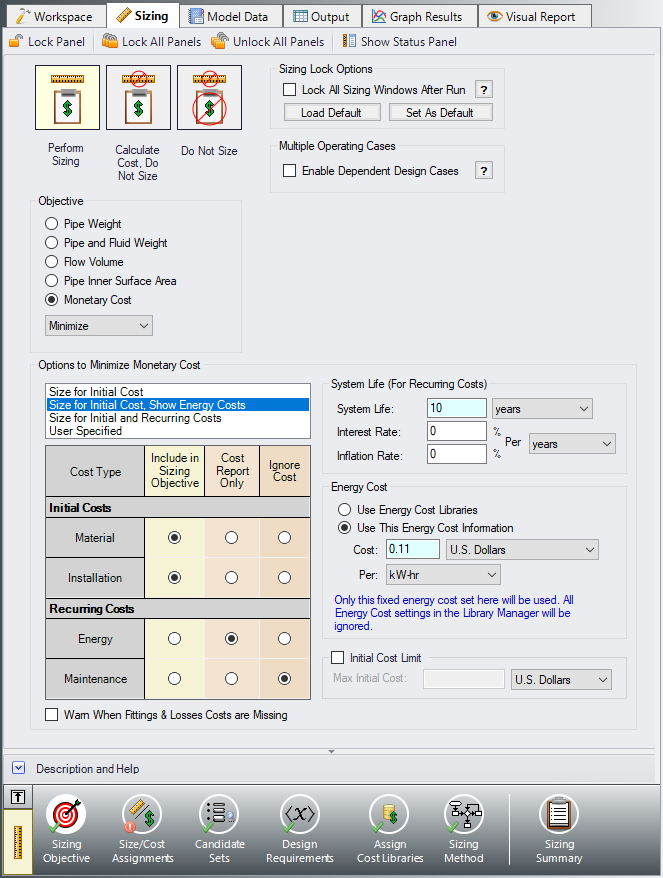
A. Sizing Objective
The Sizing Objective window should be selected by default from the Sizing Navigation panel along the bottom. For this analysis, we are interested in sizing the system considering the monetary cost for the initial costs only.
-
Sizing Option = Perform Sizing
-
Objective = Monetary Cost
-
Option = Minimize
-
Options to Minimize Monetary Cost = Size for Initial Cost, Show Energy Costs
-
This will update the cost table to include both initial costs in the sizing calculation, and moves the Energy costs to be included in the Cost Report so that we can later compare the costs in this scenario to one where the Energy costs are included for the sizing. We do not have any information on Maintenance cost, so we will leave this cost in Ignore Cost.
-
-
System Life = 10 years
-
Energy Cost = 0.11 U.S. Dollars Per kW-hr
-
Note this assumes the pump will run all day, every day, for the entire 10 years. Alternatively, we could have created an Energy Cost Library, which would be connected in the Assign Cost Libraries section. An Energy Cost Library allows variable energy costs to be used to account for varying prices during different times of day, different seasons, etc. For now, we are simplifying the input by using a fixed cost.
-
The Sizing Objective window should now appear as shown in Figure 2.
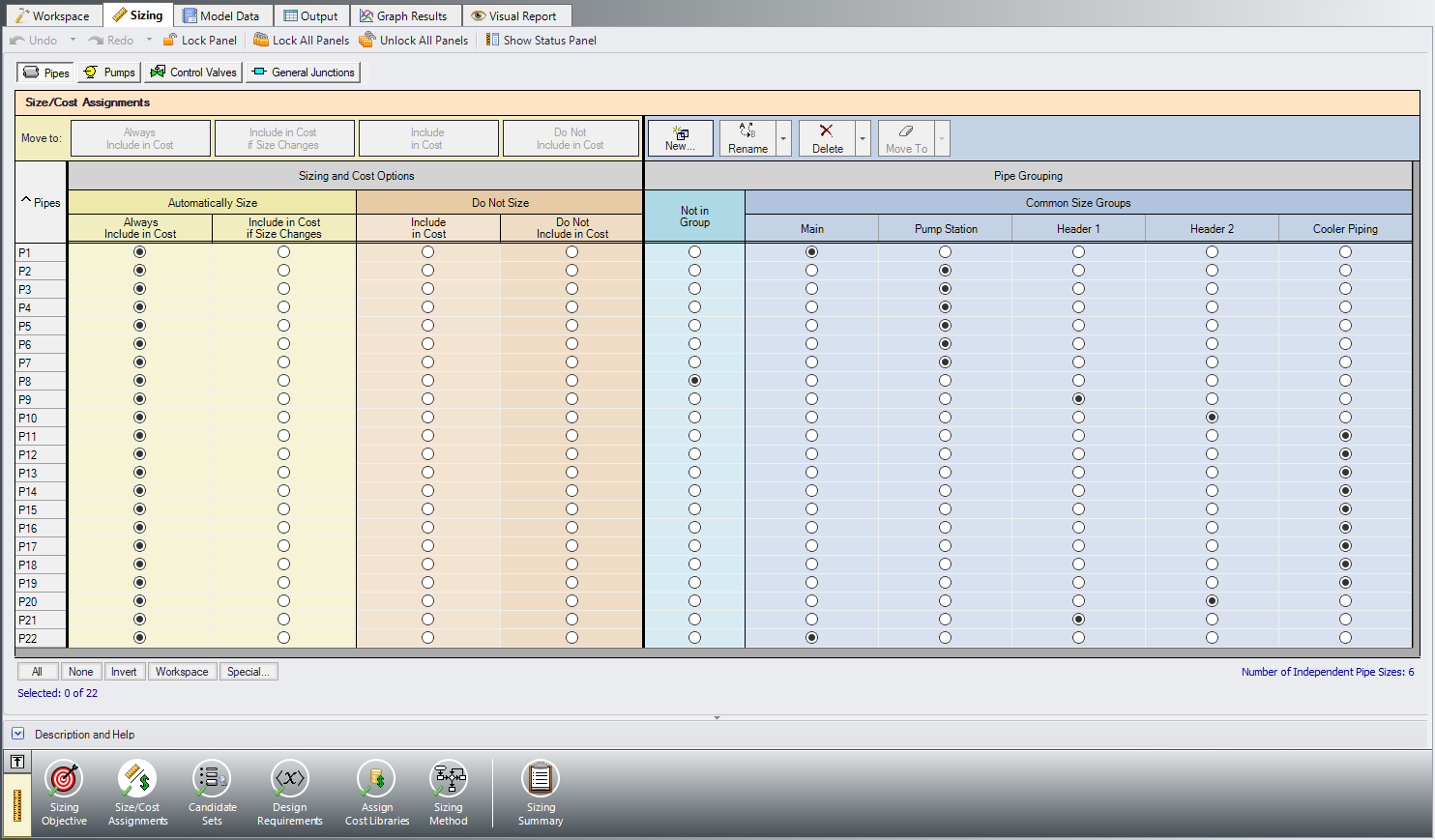
B. Size/Cost Assignments
On the Sizing Navigation panel select the Size/Cost Assignments button. For this example we are sizing both the pipes and pumps for a new system, so we will need to calculate and minimize cost for all related objects in the model.
ØClick All under the table to select all of the pipes, then click the Always Include in Cost button next to Move to. This will move all of the pipe selections to the corresponding column to be sized.
To decrease the run time and reduce complexity, as well as to enforce some design uniformity, it is useful to create Common Size Groups to link the pipes in different sections of the model.
For example, if all the 22 pipes are selected to be Not In Group, then 22 unique pipe sizes will be selected by the automatic sizing engine. That could potentially mean, for example, different suction pipe diameters in pipes 1 and 2. A similar thing would happen for discharge pipe diameters. If one wanted the suction pipes 1 and 2 to be sized to the same diameter, one would group them into a Common Size Group. To see how this works, in this model all suction and discharge piping for both pumps will be put into a Common Size Group. What this means is that there will be one unique diameter chosen for this group of pipes, rather than potentially six different diameters.
For this system we will define five groups to be sized in this model. To set the groups, it is standard to select pipes which must have the same size due to their placement relative to other pipes and junctions, such as pipes at the entrance and exit of valves. In Figure 3 we have identified the five sections of the model to group the pipes.
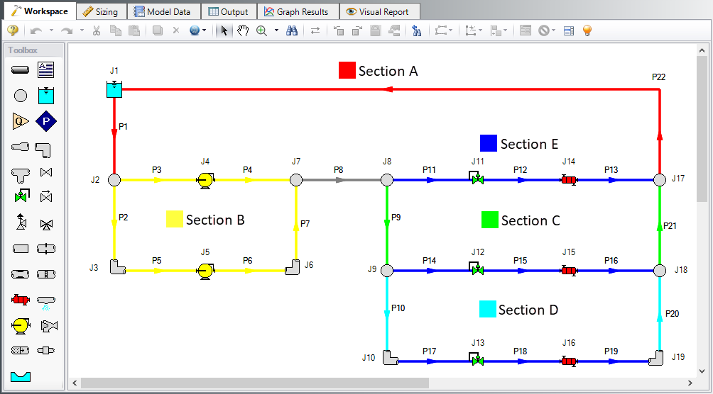
First let’s create a Main size group for pipes 1 and 22, which are blue in Section A. We would expect these lines to be sized the same, as the inlet and outlet for the cooling reservoir.
ØClick New above the Pipe Grouping section to create the group, and name it Main. Select the radio buttons under Main next to 1 and 22 to add them to the group. Alternatively, both pipes could be selected in the Workspace, then be added to a new group by right-clicking the Workspace and choosing Add Pipe(s) to Common Size Group.
Now let’s repeat this process for the piping in Section B around the pumps and control valves. Since this section contains identical pumps operating in parallel, we would expect the pipes in this section to have a common size. Similar to above, create a new group called Pump Station, and add pipes 2-7 as shown in green in Figure 3 in section B to the new group by selecting them in the Workspace, or using the radio buttons.
Next, let’s consider Section C-E, the piping near the coolers. In this case we have three coolers in parallel, with several segments of pipe connecting the cooler piping segments. We would expect the pipes directly connected to the coolers to have a common size, but the header piping (9, 10, 20, 21) would likely need to be larger, so we will group them separately. Create three Common Size Groups as follows:
-
Header 1 with 9 and 21 (Section C, magenta)
-
Header 2 with 10 and 20 (Section D, red)
-
Cooler Piping with 11-19 (Section E, orange)
The completed Size/Cost Assignments can be seen in Figure 4. Note that pipe 8 should be the only pipe not included in a group. This leaves six different pipe sizes that the ANS module will independently solve for during the automated sizing, one for each of the groups, and one for pipe 8. This is indicated in the bottom right of the Size/Cost Assignments panel, which shows that six independent pipe sizes exist for this configuration.
Note: Pipes in the Size/Cost Assignments table can be sorted by Common Size Group instead of sorting by number by clicking on the Pipe Grouping header. Clicking on the header for a particular group will sort the pipes in that specific group to the top of the window.
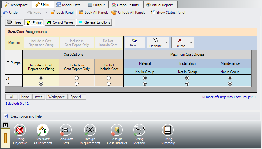
ØClick the Pumps button to switch to view the Pump Size and Cost Assignments. Select the option to Include in Cost Report and Sizing for both pumps so that the ANS module will size the pumps along with the pipes as shown in Figure 5.
Similar to the Common Size Groups for pipes, Pumps can be placed into Maximum Cost Groups based on monetary cost. If pump costs are added to a Maximum Cost Group, the ANS module will determine the pump in the group with the maximum costs, and set all pumps in the group to use the largest cost. In this case we will allow the pumps to be sized independently, so no groups need to be created.
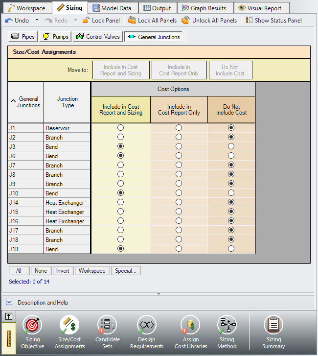
We also want to include the Bends in the sizing for this model.
ØClick the General Junctions button and change each of the Bends (3, 6, 10, and 19) to Include in Cost Report and Sizing (Figure 6)
C. Candidate Sets
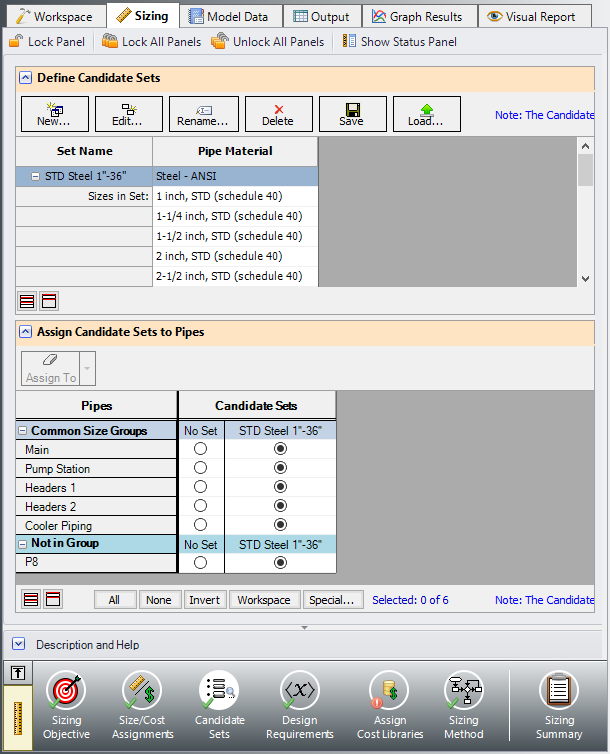
Click on the Candidate Sets button to open the Candidate Sets panel.
Click New under Define Candidate Sets and name it STD Steel 1"-36". In the Select Pipe Sizes window, select Steel - ANSI from the dropdown menu, expand the STD group (make sure the Sort selection on the bottom is Type, Schedule, Class), then add all pipes from 1 inch to 36 inch to the Candidate Set list on the right.
In the bottom section of the window, assign each of the Common Size Groups and pipe P8 to the STD Steel 1"-36" Candidate Set. The window should appear as shown in the figure below.
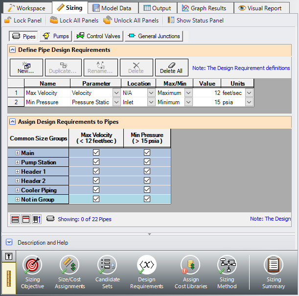
D. Design Requirements
Select the Design Requirements button from the Sizing Navigation Panel.
For this model we have multiple requirements for the system:
-
Max Velocity: All pipes have a maximum velocity of 12 feet/sec
-
Min Pressure: All pipes have a minimum static pressure requirement of 15 psia
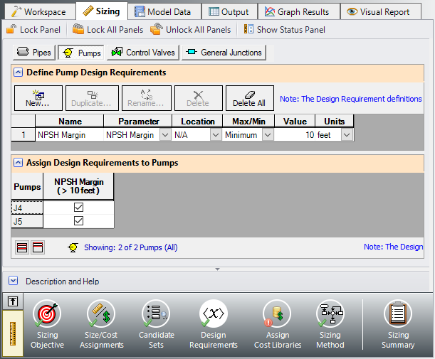
-
NPSH Margin: All pumps must have a minimum NPSH Margin of 10 feet (for this system the nominal NPSHR is 50 feet)
-
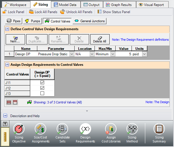
Design DP: All control valves must have a minimum static pressure drop of 5 psid
-
All heat exchangers must receive a minimum flow of 1900 gal/min
Define and assign the first two requirements listed above as Pipe Design Requirements as shown in Figure 8, and item 3 as a Pump Design Requirement as shown in Figure 9. Notice that we have accounted for the minimum flow requirement in this system by using flow control valves at each of the heat exchangers. By using assigned flow pumps and flow control valves at the heat exchangers (we will do this later) we will incorporate the necessary flow rate as a boundary condition, so we do not need to apply a Design Requirement to account for this item.
For Control Valves 9 and 13 define and apply the minimum pressure drop requirement in the Control Valves section as shown in Figure 10. Note that for pump sizing purposes as discussed earlier Control Valve 13 has been defined as a Constant Pressure Drop valve, so the pressure drop Design Requirement does not need to be applied to this valve.
E. Assign Cost Libraries
Select the Assign Cost Libraries button. For this model the engineering and cost libraries have already been created, but we will need to connect and apply them.
Note: The Cooling System, Creating Libraries - ANS example provides instructions on how to build the libraries for the first part of this example, and may be completed later for practice with creating libraries. The provided pre-built libraries will be needed to obtain the pump curve data for Step 16 of this example.
ØOpen the Library Manager by opening the Library menu and selecting Library Manager. The AFT INTERNAL LIBRARY, LOCAL USER LIBRARY, and the pipe material libraries should be available and connected by default. Available libraries will be shown based on libraries that Fathom has identified on your machine. The default connected libraries will be visible here, and additional libraries may be visible from other example files or from libraries previously built and used on your machine.
This example uses one user-defined engineering library Cooling System.dat, which contains the data for the pumps and bends. There are also two cost libraries, Cooling System Costs.cst and Steel - ANSI Pipe Costs.cst, which contain the cost data for the junctions and the pipe materials, respectively. Cooling System Costs.cst was built off of the engineering library Cooling System.dat, and Steel - ANSI Pipe Costs.cst was built off of the Steel - ANSI Pipe Material Library. To connect these libraries, do the following:
-
Click Add Existing Library.
-
Browse to the Fathom 12 Examples folder (located by default in C:\AFT Products\AFT Fathom 12\Examples\), and open the file titled Cooling System.dat.
-
Repeat the above steps, but choose Add Existing Cost Library to browse for Cooling System Costs.cst, then Steel - ANSI Pipe Costs.cst.
Note that it may be possible that the model file already has the cooling system libraries connected, in which case you will be notified that the library you are trying to add is already available. If the libraries are available, you will simply need to make sure they are connected by ensuring a checkmark is next to the name. There should be a library titled Cooling System with two sub libraries: Junctions and Cost (Cost should have a cost file titled Cooling System Costs beneath it. Additionally a Cost sub library should appear subordinate to the Steel - ANSI, the library Steel - ANSI Pipe Costs should appear beneath it.
Note: When a library is selected in the Library Manager, the filename and location can be viewed in the Selected Content Information section.
Once you have confirmed that the necessary libraries are connected, click Close to exit the Library Manager.
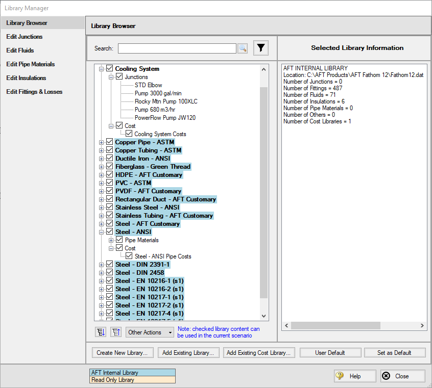
Figure 11: Library Manager with Cooling System junction libraries connected
Since we are connecting a pre-built engineering library, we will need to take an additional step to confirm that the junctions in the Workspace are linked to the Cooling System engineering library that we added.
-
Go to the Workspace, and open Pump J4
-
From the Library Jct list, select Pump
-
Repeat step 2 for Pump J5.
-
Open each of the Bends (junctions 3, 6, 10, and 19), and select STD Elbow for each from the Library Jct list, and click OK.
We have now re-connected the junctions that will be considered for the Cost Report and Sizing Calculations to the engineering library. This is important, since a junction must be connected to an engineering library before a cost can be assigned for it. Let's now return to the Sizing tab.
Back in the Assign Cost Libraries panel for the Pipes, All should be selected for the STD Steel 1"-36" inch Candidate Set with only the Steel - ANSI Pipe Costs library shown. The user can create and connect as many cost libraries as desired, which can be useful to easily update the cost of individual objects, rather than having to keep all of the costs in one large library. If multiple cost libraries are assigned to a Candidate Set, then the costs will be stacked to find a cumulative cost.
ØClick on the Pumps button to view the cost library assignments for the Pumps. The only visible library should be the Cooling System Costs library, as this was the only cost library connected for the associated engineering library. Make sure that the checkboxes are selected under the library name so that the cost data will be applied for each of the pumps. To review the cost data for the Bends click the General Junctions button to verify that the Cooling System Costs are being applied to each of the bends.
F. Sizing Method
Select the Sizing Method button to go to the Sizing Method panel.
ØChoose Discrete Sizing, if not already selected, since it is desired to select discrete sizes for each of the pipes in the model.
For this model we have six independent pipe sizes as mentioned earlier (five Common Size Groups and pipe 8), and 48 design requirements (2 pipe design requirements applied to all of the pipes, the pump NPSH requirement, and the minimum pressure drop for control valves). Due to the number of independently sized pipes, it would be recommended to try the MMFD or SQP search method. Though it is not shown here, if both methods are run for this scenario the same solution will be obtained, with the Modified Method of Feasible Directions (MMFD) being the most efficient.
Select Modified Method of Feasible Directions (MMFD) for the sizing method.
G. Sizing Summary
From the Sizing Navigation Panel select the Sizing Summary button.
The Sizing Summary panel allows the user to view all of the sizing input for the model in a tree view layout, which is shown in Figure 12. Items can be organized by sizing parameters (Design Requirements, Candidate Sets, etc.), or information can be viewed based off an individual pipe. For clarity these categories can be shown/hidden using the check boxes at the top of the panel.
Each tree node can be expanded/collapsed individually by using the ‘+’ and ‘-‘ buttons on the node. Alternatively, the buttons on the bottom of the panel can be used to collapse/expand all items. Right-clicking on the nodes provides additional options to collapse/expand items, view related nodes, or to copy information to the clipboard. The Sizing Summary panel can be printed from the printer button at the bottom of the panel.
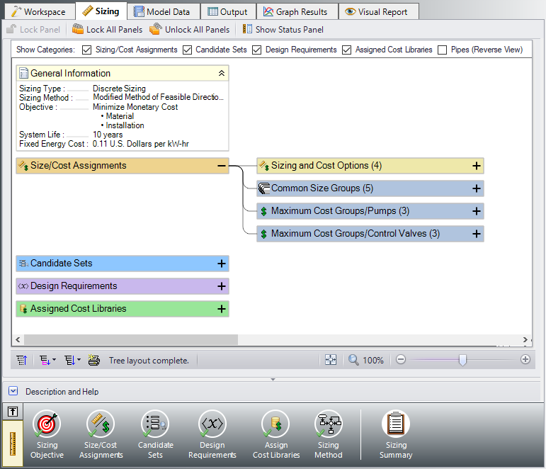
Figure 12: Sizing Summary panel layout with the Size/Cost Assignments expanded. The number of children nodes for each item can be seen in parentheses.
Step 8. Set up the Scenario Manager
To compare the four potential sizing cases, child scenarios will be set up in the Scenario Manager. Go to the Scenario Manager now and create the following child scenarios based on Figure 13 below. These will include the Not Sized scenario and the four potential sizing cases: Initial Cost, Life Cycle Cost, Initial Cost Limit, and Actual Pump Curve.
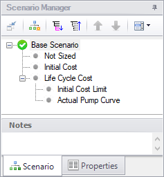
Step 9. Set up the Not Sized scenario
Load the Not Sized scenario by double-clicking on it in the Scenario Manager.
Navigate to the Sizing window and go to the Sizing Objective panel. Select Calculate Cost, Do Not Size. In the Options to Minimize Monetary Cost, the selection should be User Specified. Make sure that the radio buttons for Material, Installation, and Energy are selected for Cost Report Only, while Maintenance should have Ignore Cost selected.
This will calculate the life cycle cost of the system before any sizing is performed. This cost will be used as a comparison to the sized scenarios.
Step 10. Run the Model
Select Run Model in the Analysis menu. This will open the Solution Progress window. This window allows you to watch as the Fathom Solver and ANS module converge on a solution.
After the run has been completed, the results can be reviewed clicking the Output button at the bottom of the solution progress window.
Step 11. Review the Not Sized results
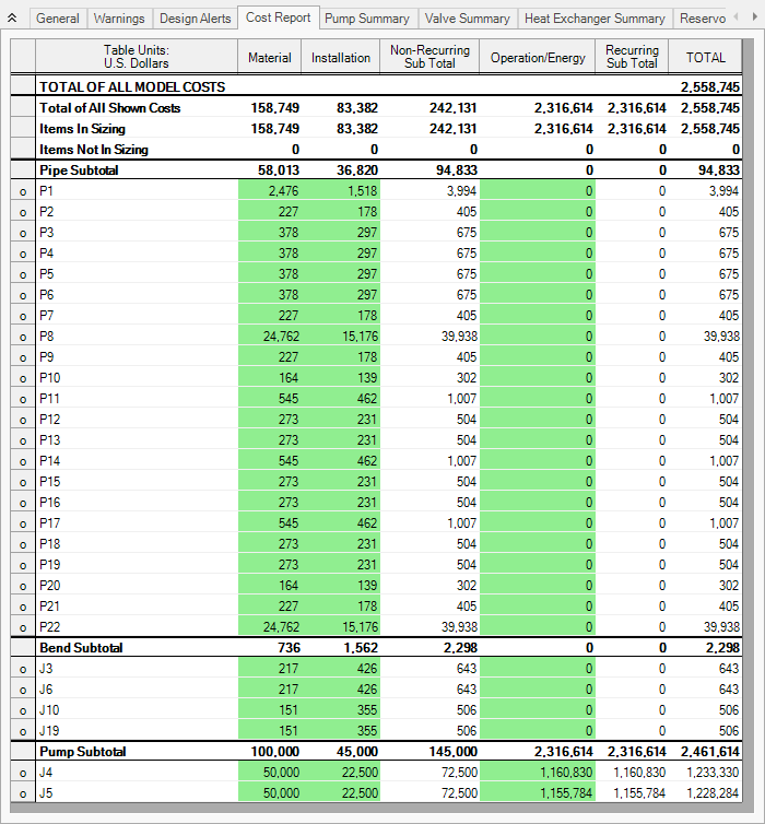
The Cost Report is shown in the General Section of the Output window (see Figure 14). No sizing was performed, so all cost values will appear in the Items Not In Sizing row. The total cost for this system is
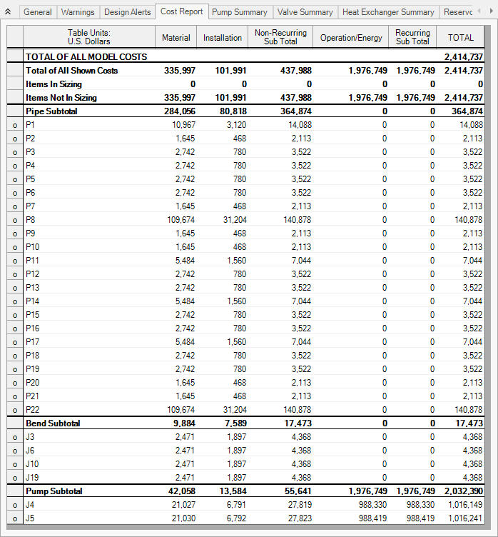
Figure 14: The Cost Report in the Output window shows the total and individual costs (in thousands of U.S. Dollars) for the sized system
With this basis, we will move on to the Initial Cost scenario.
Step 12. Run the Initial Cost scenario and review the results
Load the Initial Cost scenario using the Scenario Manager. This scenario should have all the inputs already specified, so no action is required besides running the model.
Click Run Model on the toolbar or from the Analysis menu. When finished, view the results by clicking the Output button at the bottom of the Solution Progress window.
Go to the Cost Report, as shown in Figure 15. ANS shows all costs in the Cost Report, including those that were not used in the automated sizing. The total cost for this system is
Other costs that are displayed in the Cost Report are Items Not in Sizing. These are items that have costs associated with them, but were not included in the automated sizing.
Note that the Items Not in Sizing total to
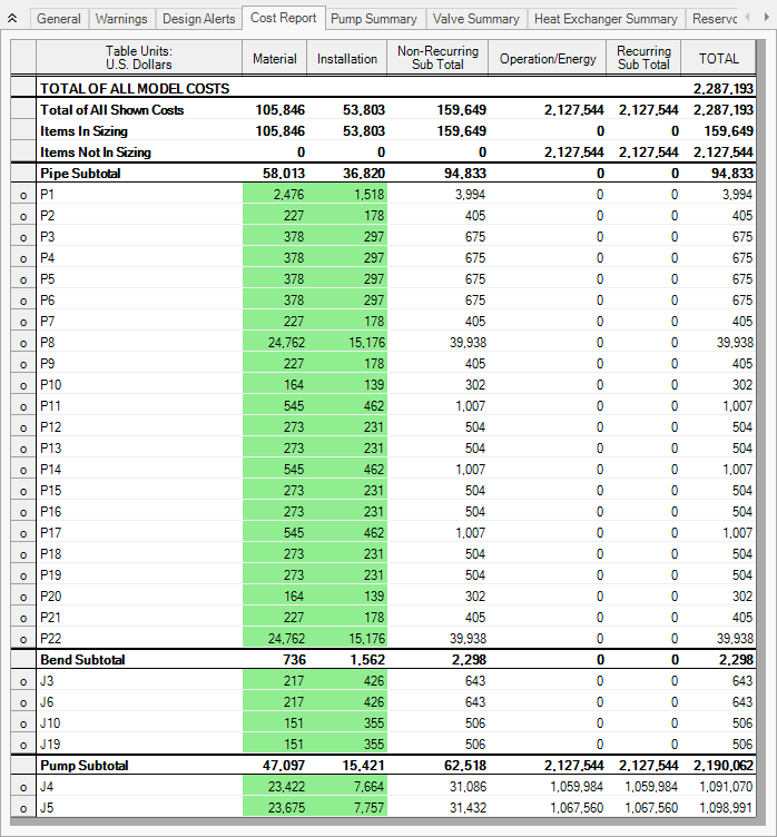
Figure 15: The Cost Report in the Output window shows the total and individual costs (in thousands of U.S. Dollars) for the sized system
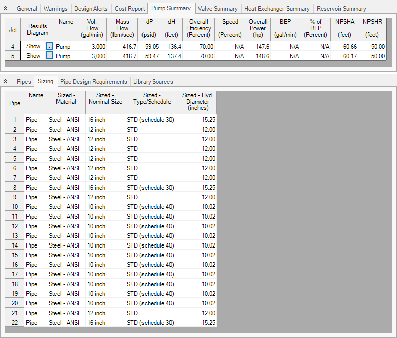
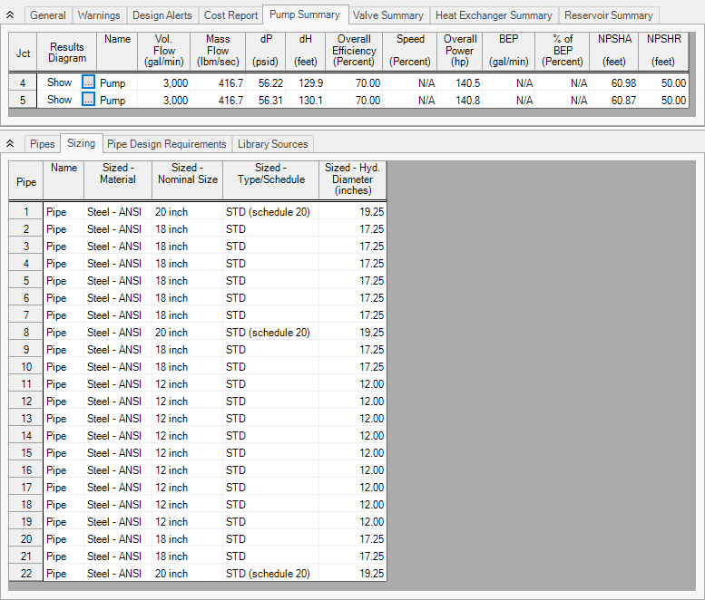
In the Pipes section of the Output window the final pipe sizes from the automated sizing can be seen, along with the Design Requirements status. For this model, the final system used pipe sizes varying from 10 to 16 inches, as seen in Figure 16. The information for the pumps can be seen in the Pump Summary tab in the General Section, which is also shown in Figure 16.
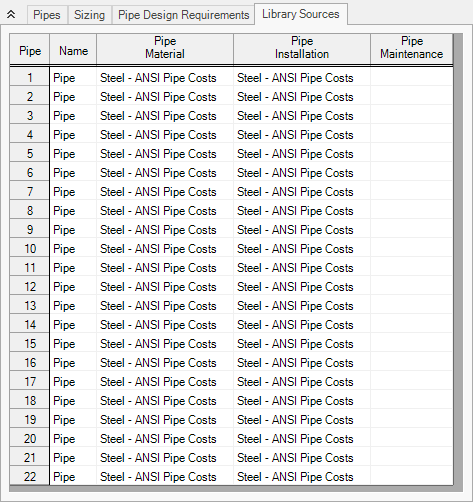
When a monetary cost objective is selected, additional tabs are available that display the Library Sources used for the Cost Report for each of the pipes/junctions. In this case both the Pipe Material and Pipe Installation costs for all of the pipes came from the Steel - ANSI Pipe Costs library which was connected earlier. Information for the Pumps and Bends came from the Cooling System Costs library. If multiple cost libraries are used for a category they will all be listed separated by commas. The Library Sources for the Pipes can be seen in Figure 17.
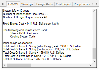
On the General tab of the Output window at the bottom of the report, the initial cost of the items included in the sizing can be seen, which was
Although there was a 63% reduction in initial costs, the total cost decreased by 5%. Next, we will see how much more the total cost can be reduced by doing a life cycle system sizing.
Step 13. Size System for Life Cycle Cost over 10 Years
Load the Life Cycle Cost scenario from the Scenario Manager. Go to the Sizing window, and make sure that the Sizing Objective panel is opened. Under Options to Minimize Monetary Cost, choose Size for Initial and Recurring Costs. This will move the Energy costs selection to Include in Sizing Objective. The scenario is now complete.
ØClick Run from the Analysis menu to run the automated sizing. When the calculations have finished, click Output to view the results.
Step 14. Compare the Sizing Results
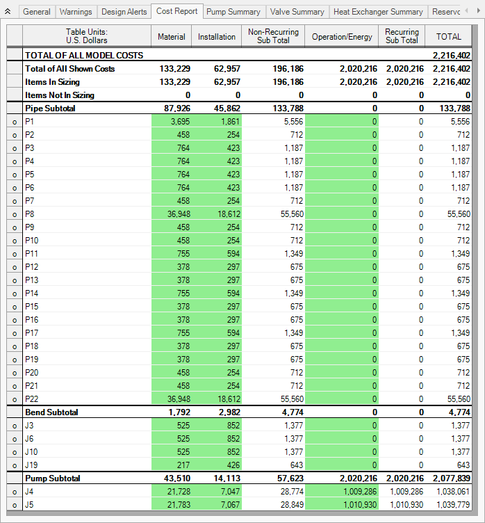
After viewing the Cost Report, it can be seen that the total cost is now
Taken on its own, this new cost represents a savings of about $198,000 (8%) compared to the Not Sized scenario. Compared to the Initial Cost scenario, which was sized to minimize initial cost only, this new scenario represents a savings of $71,000. This represents a total 3% cost reduction. In the Initial Cost scenario, the non-recurring cost was $159,649, while the overall cost was $2,287,193. Now the non-recurring cost is $196,186 while the overall cost is $2,216,402. The initial cost thus increased by about $36,500 in order to reduce the operating cost from $2,127,544 to $2,020,216 (a reduction of about $107,000). The source of the operating cost is the cost of power for the pumps. To reduce pump power usage, it makes sense to increase the pipe size and thus reduce frictional losses. The larger pipe sizes can be reviewed by looking at the Sizing tab in the Pipe Output section. From the Pump Summary tab it can be seen that the pump power usage decreased from 148 to 141 hp at each of the pumps, which is approximately a 5% power requirement decrease at each pump. The Pump Summary and final pipe sizes can be seen in Figure 20.
Considering this cost breakdown between the scenarios highlights the importance of choosing to include the energy costs in the initial cost scenario. If they were not in the Cost Report of the initial cost scenario, the total cost would be
By performing both analyses the designer has quantitative data on the impact of initial cost design on operational costs of the system, and can make an informed design choice.
Step 15. Size System for Life Cycle Cost with Initial Cost Limit
While the energy cost savings from life cycle cost sizing are desirable, the budget for the project may not support the higher initial cost that is required. In that case, we can apply an initial cost limit to the life cycle cost sizing.
Load the Initial Cost Limit scenario from the Scenario Manager.
ØReturn to the Sizing Objective panel and select the option for Size for Initial and Recurring Costs and check the box next to Initial Cost Limit. We will set the limit as $175,000, which is slightly more than the initial cost of the scenario that minimized initial cost at the expense of an increased life cycle cost. Run the model and go to the Output tab.
A summary of the results with the initial cost limit compared to each of the initial and life cycle cost sizing scenarios for a 10 year life cycle can be seen in Table 1.
Notice that while the material and installation costs were limited to $175,000, the total costs over a 10 year lifetime are decreased by about
Table 1: Cost Summary of Sizing Runs for Cooling System
| Scenario | Material | Installation | Non-Recurring Sub Total | Operation/Energy | TOTAL | Reduction |
|---|---|---|---|---|---|---|
| Not Sized | 335,997 | 101,991 | 437,988 | 1,976,749 | 2,414,737 | - |
| Initial Cost | 105,846 | 53,803 | 159,649 | 2,127,544 | 2,287,193 | 127,544 |
| Life Cycle Cost | 133,229 | 62,957 | 196,186 | 2,020,216 | 2,216,402 | 198,335 |
| Initial Cost Limit | 117,565 | 57,808 | 175,373 | 2,058,223 | 2,233,596 | 181,141 |
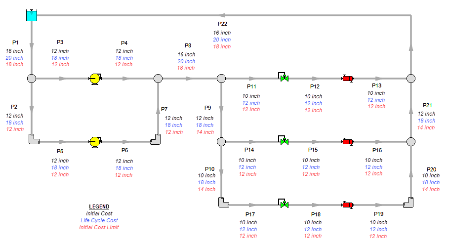
Figure 21: Pipe sizes selected by the ANS module for initial cost and life cycle cost with an initial cost limit compared to the original design. Note that this diagram was generated outside of AFT Fathom.
Step 16. Automated Sizing with Pump Curve Data
As discussed in the section Summarizing the pump selection process, once the pump is sized then actual pumps can be modeled. The actual pump should closely match the sizing results in the following areas: generated head at the design flow, efficiency at the design flow, and cost. We will apply a pump curve for the case that was sized for life cycle cost to complete the pump selection process.
Reviewing the results for the life cycle cost scenario one can see that the sized system calls for a pump of about
Based on the sizing analysis, we will choose a pump from the (fictitious) Rocky Mountain Pump Company. Its model 100XLC is a close match for the requirements of a 10-year life cycle design. The model 100XLC has the following characteristics: at 3,000 gal/min its head is 135 feet and efficiency is 70%. Its material cost is $50,000 and installation cost is $22,500. To set up a new scenario for the system with the candidate pump data:
-
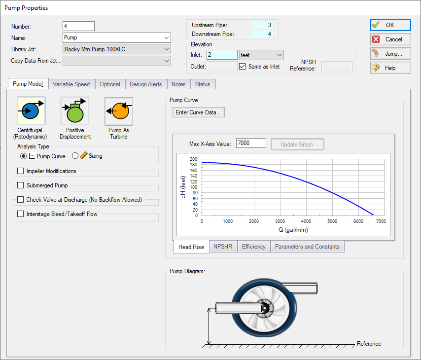
Load the Actual Pump Curve scenario and go to the Workspace. In the properties window for each of the pumps select
-
In the Control Valve properties window for J13, change the Valve Type to Flow Control (FCV), and enter a Flow Setpoint of
-
Go to the Sizing window, navigate to the Design Requirements panel, select the Control Valves button at the top of the window, and apply the Design DP design requirement to J13.
The necessary changes are now complete to size the system with the updated pump and flow control valve data.
ØSelect Run from the Analysis menu to perform the automated sizing - this may take some time.
When the solver has finished, click Output to review the results. The overall cost for the system is about
Now we have sized the system for use with an actual pump.