Hot Water System - ANS (English Units)
Hot Water System - ANS (Metric Units)
Summary
This example will take an existing hot water system design, scale it up, and size the pipes to meet a set of system requirements at a minimal cost. The system cost is included to demonstrate the need for sizing. The system must meet the following requirements:
-
Minimum 10 psid drop across flow control valves in all cases
-
Maximum 8 feet/sec velocity in all pipes in all cases
-
No NPSH violations
-
All pumps must operate between 80% to 100% of the BEP (Best Efficiency Point)
-
System must also function with Pump A turned off with no BEP restrictions
-
The flow rate through the heat exchangers is controlled by FCVs set to 3,000 gal/min.
Note: This example can only be run if you have a license for the ANS module.
Topics Covered
-
Defining pump Design Requirements
-
Sizing the system to minimize initial costs
-
Using Dependent Design Cases
Required Knowledge
This example assumes the user has already worked through the Walk-Through Examples section, and has a level of knowledge consistent with the topics covered there. If this is not the case, please review the Walk-Through Examples, beginning with the Beginner: Three Reservoir Model example. You can also watch the AFT Fathom Quick Start Video Tutorial Series on the AFT website, as it covers the majority of the topics discussed in the Three-Reservoir Model example.
In addition, it is assumed that the user has worked through the Beginner: Three-Reservoir Problem - ANS example, and is familiar with the basics of ANS analysis.
Model Files
This example uses the following files, which are installed in the Examples folder as part of the AFT Fathom installation:
-
Hot Water System.dat - engineering library
-
Hot Water System Costs.cst - cost library for Hot Water System.dat
-
Steel - ANSI Pipe Costs.cst - cost library for Steel - ANSI pipes
Step 1. Start AFT Fathom
From the Start Menu choose the AFT Fathom 12 folder and select AFT Fathom 12.
To ensure that your results are the same as those presented in this documentation, this example should be run using all default AFT Fathom settings, unless you are specifically instructed to do otherwise.
Step 2. Open the model
Open the
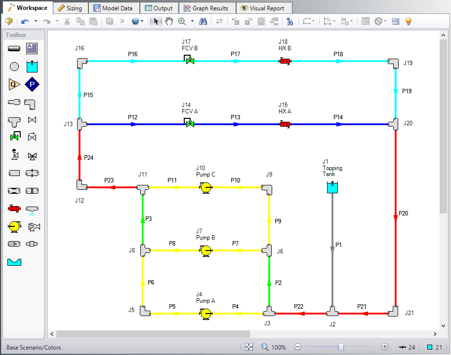
Although the model is fully defined, a few alterations are necessary for this example to scale up the system. First make sure that the Workspace looks like Figure 1 below, though the pipes will not be colored:
Step 3. Define the Modules Panel
Open Analysis Setup from the toolbar or from the Analysis menu. Navigate to the Modules panel. For this example, check the box next to Activate ANS and select Network to enable the ANS module for use. A new group will appear in Analysis Setup titled Automatic Sizing. Click OK to save the changes and exit Analysis Setup. A new Primary Window tab will appear between Workspace and Model Data titled Sizing. Open the Analysis menu to see the new option called Automatic Sizing. From here you can quickly toggle between Not Used mode (normal AFT Fathom) and Network (ANS mode).
Step 4. Define the Pipes and Junctions Group
For this example, the existing system is being scaled up. As an initial design, set all pipe diameters to 20 inches and increase the flow setpoints of the control valves to
Make the following changes to these pipes junctions
-
All Pipes
-
Size = 20 inch
-
Type = STD (schedule 20)
-
-
J14 & J17 Control Valves
-
Flow Setpoint = 3000 gal/min
-
Step 5. Configure Sizing Settings
We will need to define the sizing settings to account for the three given Design Requirements while minimizing the initial costs for the system. To do this, we will follow the Sizing steps as outlined below.
A. Sizing Objective
The Sizing Objective panel should be selected by default in the Sizing Navigation panel.
Select Perform Sizing.
For the Objective, make sure that Monetary Cost is selected, and Minimize is chosen from the drop-down.
We will also need to specify which types of monetary cost we want to size for. Choose Size for Initial and Recurring Costs, if not selected already, to move the Material and Installation costs to the column to be sized.
Set the System Life to 10 years.
Under Energy Cost, select Use This Energy Cost Information and enter 0.10 U.S. Dollars Per kW-hr.
B. Size/Cost Assignments
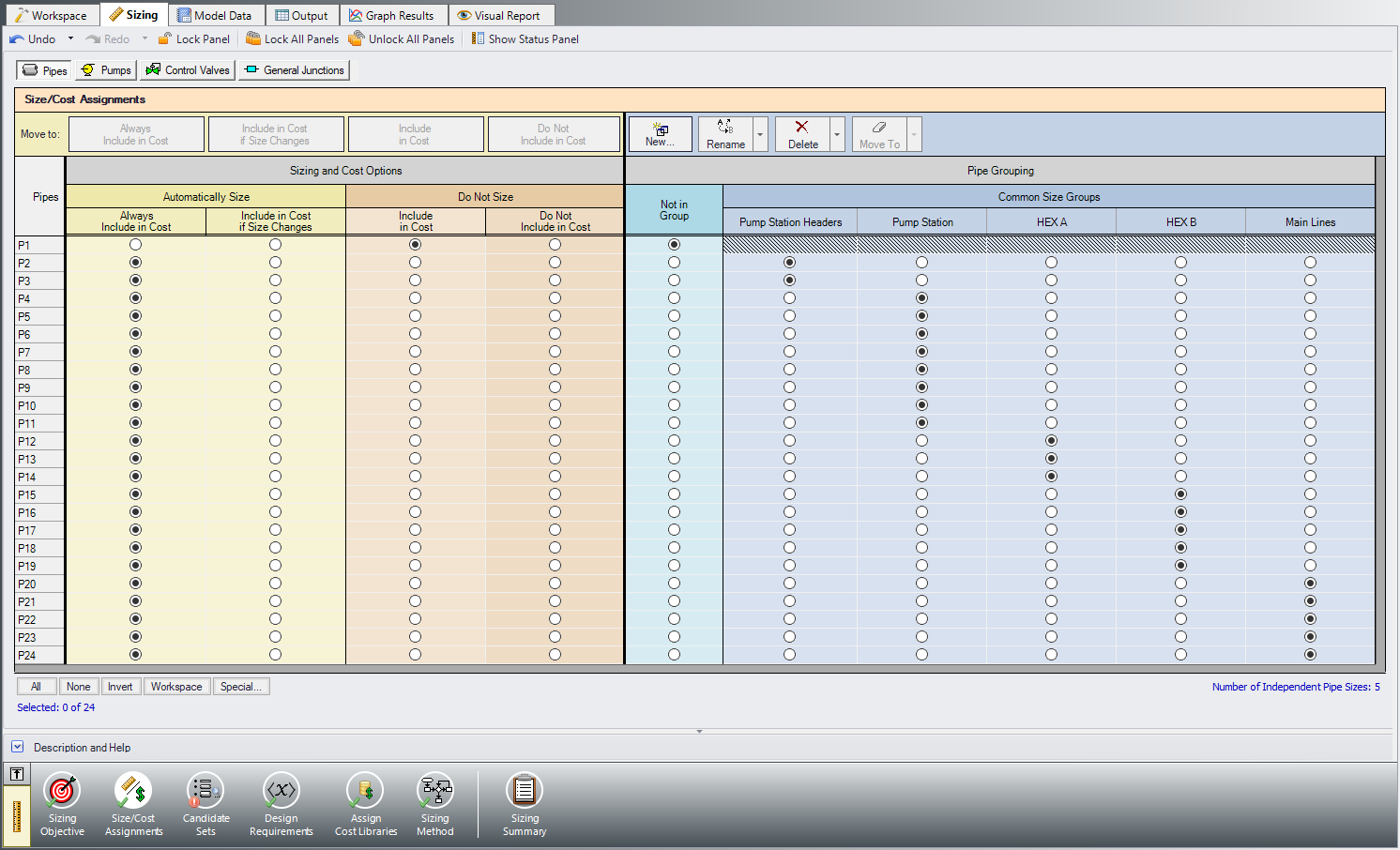
On the toolbar at the bottom of the window select the Size/Cost Assignments button. The Size/Cost Assignments window allows the user to define what will be sized in the model.
To increase the analysis speed and reduce complexity, it is useful to create Common Size Groups to group the pipes in different sections of the model. For this system we have defined 5 groups to be sized, as can be seen in Figure 2. We do not want to size pipe P1, but we will include it in the cost calculation for the sake of comparison later.
ØCreate the Common Size Groups shown in Figure 1 and Figure 2 in the model by either using the radio buttons in the table, or by selecting the pipes in the Workspace and adding them to groups from the right click menu.
Besides the pipes, it is also desired to include the pumps in the sizing.
ØSelect the Pumps button then set each of the pumps to be included in the Cost Report and Sizing.
C. Candidate Sets
Click on the Candidate Sets button to open the Candidate Sets panel.
Click New under Define Candidate Sets and name it STD Steel 1"-36". In the Select Pipe Sizes window, select Steel - ANSI from the dropdown menu, expand the STD group (make sure the Sort selection on the bottom is Type, Schedule, Class), then add all pipes from 1 inch to 36 inch to the Candidate Set list on the right.
In the bottom section of the window, check that each of the Common Size Groups have been assigned to use the existing Candidate Set.
D. Design Requirements
Select the Design Requirements button.
For this model we only have three given Design Requirements which will need to be applied for the pipes, control valves, and pumps. We will start with the pipes:
-
Ensure the Pipes button at the top of the window is selected.
-
Click the New button under Define Pipe Design Requirements.
-
Enter a name when prompted: Max Pipe Velocity.
-
In the table, select Velocity as the Parameter.
-
Choose Maximum for Max/Min, and enter 8 feet/sec.
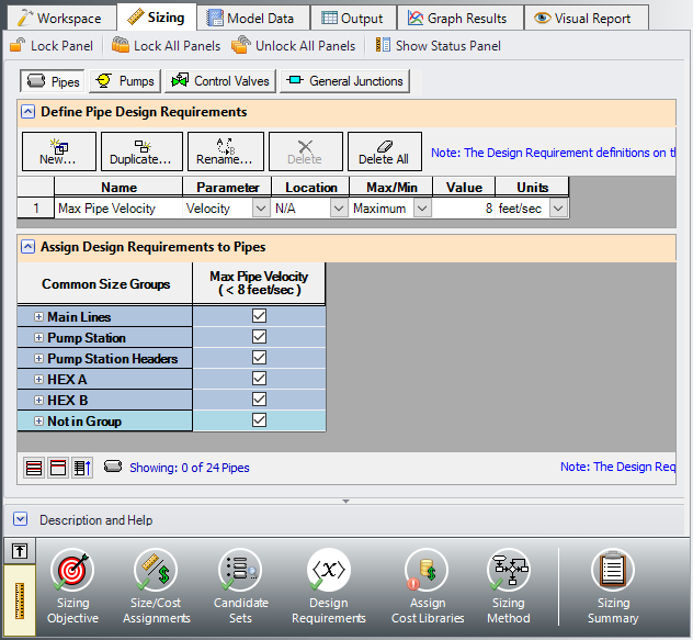
Now that the requirement is defined, make sure that it has been applied to all pipes in the model by checking the box next to each of the Common Size Groups in the bottom section of the window, as shown in Figure 3.
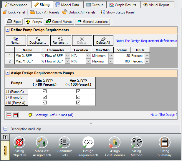
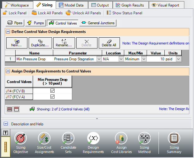
Repeat the same process as above by clicking the Control Valve, then Pump button to apply the Design Requirements for the Control Valves and Pumps as follows, and as is shown in Figure 5 and Figure 4 respectively.
-
All of the Pumps must have a minimum % Flow of BEP of 80% and a maximum % Flow of BEP of 100%
-
Both Control Valves must have a minimum stagnation pressure drop of 10 psid
Note: The Design Requirements are not enforced when the model is not being sized. Instead, the design requirements are treated as Design Alerts, which is useful to assess the feasibility of the initial design.
E. Assign Cost Libraries
Select the Assign Cost Libraries button. For this model the engineering and cost libraries have already been created, but we will need to check that they have been connected and applied properly.
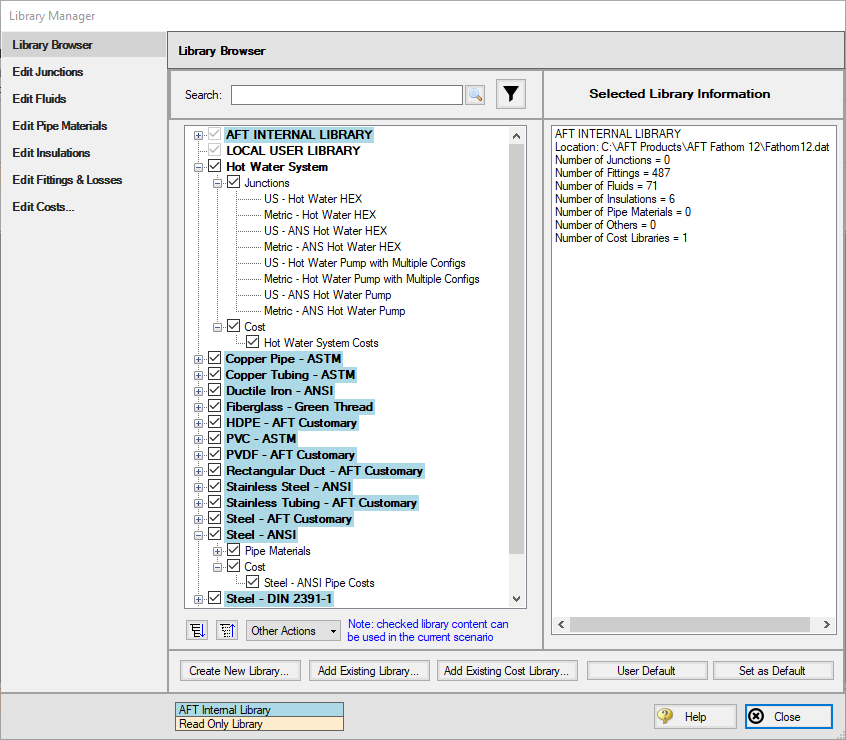
ØOpen the Library Manager by clicking the Library Manager button to see which libraries are connected. The AFT INTERNAL LIBRARY and LOCAL USER LIBRARY should be available and connected. The AFT internal library also has a cost library associated with it. This example uses the engineering library Hot Water System.dat and two cost libraries, Hot Water System Costs.cst and Steel - ANSI Pipe Costs.cst which are linked with the Hot Water System engineering library and the pipe material library for Steel - ANSI, respectively. If the libraries are connected, there will be a check in the box next to their name, as shown in Figure 6.
If they are not in the available library list, add them from the Examples folder in the AFT Fathom 12 folder. Click Add Existing Library to navigate to and select the library Hot Water System.dat. Next, click Add Existing Cost Library and add Hot Water System Costs.cst and Steel - ANSI Pipe Costs.cst.
The
Once they have been added to the list, check to see that they are also connected. If they are not automatically connected, click the check box next to their name to connect them as seen in Figure 6. Click Close.
Back in the Assign Cost Libraries window for the Pipes, the STD Steel Pipe 1"-36" Candidate Set should now show the Steel - ANSI Pipe Costs library applied to it.
Navigate to the Workspace and connect all three pump junctions to the
Back in the Sizing window on the Assign Cost Libraries panel, click on the Pumps button to view the cost library assignments for the Pumps. Similar to the Pipes, the Hot Water System Costs library should be selected for Pumps 4, 7, and 10, showing that it is being applied.
F. Sizing Method
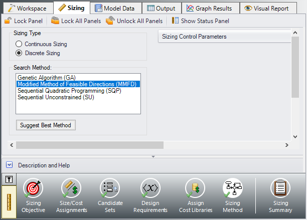
Select the Sizing Method button from the Sizing Navigation panel.
Make sure that Discrete Sizing is selected for the Sizing Type.
For this model both the Modified Method of Feasible Directions (MMFD) and the Sequential Quadratic Programming (SQP) methods will produce the same results, but MMFD is much faster. Select MMFD for the Search Method.
Step 6. Create Scenarios
For this system we would like to get a baseline cost for the current design to compare against the sizing results.
In the Scenario Manager in the Quick Access Panel create two scenarios and name them Before Sizing and After Sizing.
Load the Before Sizing scenario if it is not already active by double-clicking the scenario name in the Scenario Manager. We need to set this scenario to calculate costs without sizing the system.
In the Sizing window go to the Sizing Objective panel, then select Calculate Cost, Do Not Size.
Step 7. Run the Model
Click Run Model on the toolbar or from the Analysis menu. This will open the Solution Progress window. This window allows you to watch as the AFT Fathom solver converges on the answer. This model runs very quickly. Now view the results by clicking the Output button at the bottom of the Solution Progress window.
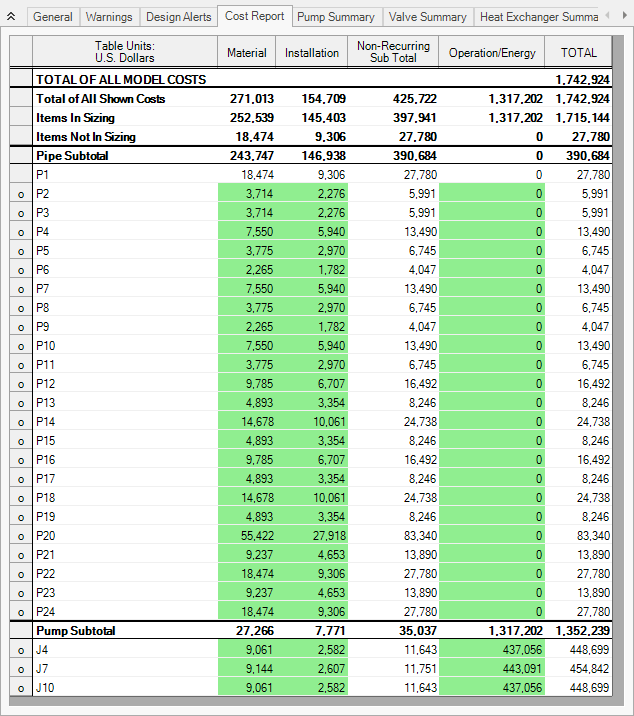
Step 8. Review the Results
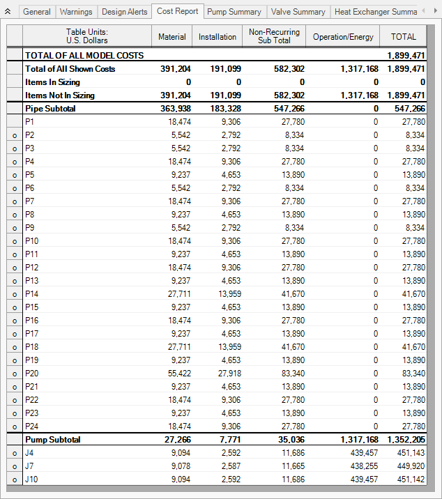
The Cost Report for the initial design can be seen in Figure 8. The total cost comes out to
Step 9. Run the Model and View Results
Switch to the After Sizing scenario in the Scenario Manager. This scenario should already be fully defined for sizing.
Select Run from the Analysis menu to perform the automated sizing calculations. Using the MMFD method, the automated sizing takes about 2 minutes, depending on your machine. When the run has completed click Output to view the results, as shown in Figure 9.
The automated sizing has given us savings of about
Step 10. Create Dependent Design Case
We also want the system to function with one pump turned off. To size a system with two different operating cases, we can create a Dependent Design Case that has the exact same pipes and junctions as the primary design but has a different set of requirements.
Create a new child of the After Sizing scenario in the Scenario Manager, and name it Sizing with Pump A off.
Here are the steps to create this Dependent Design Case:
-
Go to the Sizing Objective panel and check the box next to Enable Dependent Design Cases option.
-
Go to the Dependent Design Cases panel. You should now see instructions displayed to create the Dependent Design Case, along with a summary table of dependent design settings. Now go to the Workspace and choose Select All from the Edit menu.
-
Open Duplicate Special from Edit menu, enter an increment of 100 and select Make Dependent Design Case.
-
Click OK, then paste the duplicated model so that it does not overlap the original.
-
When the Workspace has been duplicated, select the Pump A from the Dependent Design Case (J104). In the Pump Properties window select the Optional tab and check the Pump Off No Flow radio button under Special Conditions. This will turn Pump A off.
We have now made all of the changes required in the Workspace. We will also need to make some adjustments to the Design Requirements for our Dependent Design Case. With Pump A turned off we no longer require any of the pumps to operate between 80% and 100% of BEP. We will therefore need to remove the Pump Design Requirements.
ØGo to the Design Requirements panel and select the Pumps button. In the Assign Design Requirements to Pumps section, remove the Design Requirements for all of the dependent design pumps by unchecking the boxes as is shown in Figure 10.
Once this is done run the model again and go to the Output window.

Summary
Table 1 compares the results for each of the scenarios. The final design is the lowest cost that meets all the requirements. It can be seen that in order to meet the system requirements for the case where Pump A is turned off, slightly larger pipe sizes are used, resulting in a higher system cost.
The Final Design provides a $136,000 (7%) cost reduction from the Initial Design while still meeting all design requirements.
Table 1: Summary of costs for Hot Water System scenarios
| Design Stage |
Initial Design |
Design |
Final Design |
|---|---|---|---|
| Scenario | Before Sizing | After Sizing | Sizing with Pump A off |
| Meets all Requirements | Yes | Yes | Yes |
| Material | 391,204 | 271,013 | 286,068 |
| Installation | 191,099 | 154,709 | 159,651 |
| Non-Recurring Sub Total | 582,302 | 425,722 | 445,719 |
| Operation/Energy | 1,317,168 | 1,317,202 | 1,317,224 |
| TOTAL | 1,899,471 | 1,742,924 | 1,762,942 |


