Fixed Head Supply Tank - GSC XTS (English Units)
Fixed Head Supply Tank - GSC XTS (Metric Units)
Summary
Previous examples have illustrated how to use each of the AFT Fathom modules by themselves. However, AFT Fathom also allows you to use the modules together, in any combination you choose. This allows even greater flexibility in the types of analyses that can be accomplished using AFT Fathom.
This example shows how the GSC and XTS modules and cost calculations can be performed simultaneously by examining a fixed head supply tank system.
A process plant requires the delivery of water at a fixed head, regardless of the system demand. This is accomplished by pumping the water to a supply reservoir, and maintaining a constant fill-level by varying the supply pump speed as the process demands change. Throughout any 24-hour period the process demands vary from as little as
Use the GSC and XTS modules to analyze the system performance over a 24-hour period. Perform cost calculations to determine the energy costs for the pump with this daily operation over one year.
Note: This example can only be run if you have licenses for the GSC and XTS modules.
Topics Covered
-
Using the GSC and XTS modules and performing cost calculations simultaneously
Required Knowledge
This example assumes the user has already worked through the Beginner: Three Reservoir Problem example, or has a level of knowledge consistent with that topic. You can also watch the AFT Fathom Quick Start Video Tutorial Series on the AFT website, as it covers the majority of the topics discussed in the Three-Reservoir Problem example.
In addition, it is assumed that the user has worked through the Beginner: Filling a Tank - XTS example, the Beginner: Heat Transfer in a Pipe - GSC example, and the Controlled Heat Exchanger Temperature example and is familiar with the basics of GSC, XTS module, and cost calculation analyses.
Model Files
This example uses the following files, which are installed in the Examples folder as part of the AFT Fathom installation:
Step 1. Start AFT Fathom
From the Start Menu choose the AFT Fathom 12 folder and select AFT Fathom 12.
To ensure that your results are the same as those presented in this documentation, this example should be run using all default AFT Fathom settings, unless you are specifically instructed to do otherwise.
Step 2. Define the Modules Panel
Open Analysis Setup from the toolbar or from the Analysis menu. Navigate to the Modules panel. For this example, check the box next to Activate GSC and Activate XTS. Make sure Use is selected for GSC and Transient is selected for XTS. Two new groups will appear in Analysis Setup titled Goal Seek and Control and Transient Control. Click OK to save the changes and exit Analysis Setup. Open the Analysis menu to see the two new options called Goal Seek & Control and Time Simulation. From here you can quickly toggle between Ignore (normal AFT Fathom) and Use (GSC mode) for GSC and between Steady Only (normal AFT Fathom) and Transient (XTS mode).
Step 3. Define the Fluid Properties Group
-
Open Analysis Setup from the toolbar or from the Analysis menu.
-
Open the Fluid panel then define the fluid:
-
Fluid Library = AFT Standard
-
Fluid = Water (liquid)
-
After selecting, click Add to Model
-
-
Temperature = 70 deg. F
-
Step 4. Define the Pipes and Junctions Group
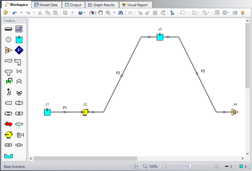
At this point, the first two groups are completed in Analysis Setup. The next undefined group is the Pipes and Junctions group. To define this group, the model needs to be assembled with all pipes and junctions fully defined. Click OK to save and exit Analysis Setup then assemble the model on the workspace as shown in the figure below.
Pipe Properties
-
Pipe Model tab
-
Pipe Material = Steel - ANSI
-
Pipe Geometry = Cylindrical Pipe
-
Size = 5 inch
-
Type = STD (schedule 40)
-
Friction Model Data Set = Standard
-
Lengths =
-
| Pipe | Length (feet) |
|---|---|
| 1 | 30 |
| 2 | 500 |
| 3 | 100 |
Junction Properties
-
J1 Reservoir
-
Tank Model = Infinite Reservoir
-
Liquid Surface Elevation = 30 feet
-
Liquid Surface Pressure = 1 atm
-
Pipe Depth = 30 feet
-
-
J2 Pump
-
Inlet Elevation = 0 feet
-
Pump Model = Centrifugal (Rotodynamic)
-
Analysis Type = Pump Curve
-
Enter Curve Data =
-
| Volumetric | Head | Efficiency |
|---|---|---|
| gal/min | feet | Percent |
| 0 | 500 | 0 |
| 1250 | 60 | |
| 2500 | 480 | 80 |
| 3750 | 70 | |
| 5000 | 250 | 40 |
-
Curve Fit Order = 2
-
J3 Reservoir
-
Name = Supply Tank
-
Tank Model = Finite Open Tank
-
Known Parameters Initially = Liquid Surface Level & Surface Pressure
-
Cross-Sectional Area = Constant, 314 feet2
-
Liquid Level Specification = Height from Bottom
-
Liquid Height = 15 feet
-
Liquid Surface Pressure = 1 atm
-
Tank Height = 20 feet
-
Pipe Depth = 15 feet
-
Tank Bottom Elevation = 20 feet
-
-
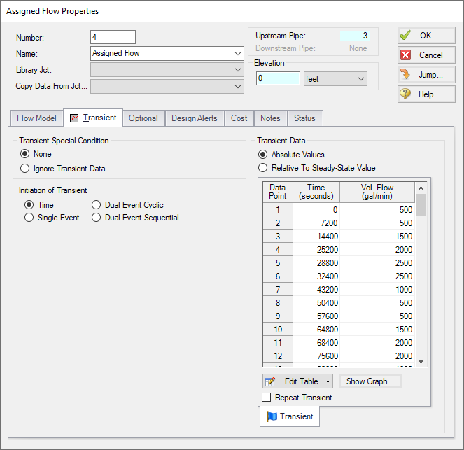
J4 Assigned Flow
-
Elevation = 0 feet
-
Type = Outflow
-
Flow Specification = Volumetric Flow Rate
-
Flow Rate = 500 gal/min
-
Step 5. Define the Goal Seek and Control Group
Specify the variables and goals for the model.
Variables Panel
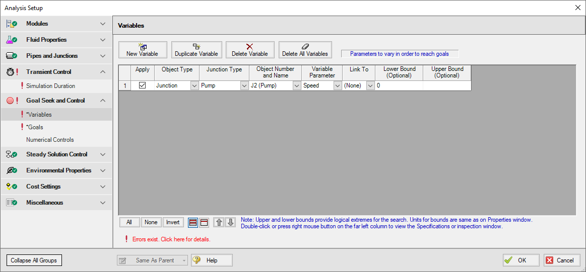
Open the Variables panel in the Goal Seek and Control group in Analysis Setup. For this example, we will be adding one pump variable: pump speed.
Click New Variable and change the Junction Type to Pump. By default, J2 (Pump) and Variable Speed will be selected for Object Number and Name and Variable Parameter, respectively. The Variables panel should look now like Figure 2.
Goals Panel
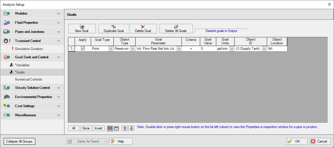
Navigate to the Goals panel. The desired goal is for the net volumetric flow rate into the junction to be zero, which will keep the water level in the tank constant.
Click New Goal and change the Object Type or Reservoir. By default, Vol. Flow Rate New Into Jct should be the selected Goal Parameter. Enter 0 as the Goal Value and select J3 (Supply Tank) for the Object ID. The Goals panel should now look like Figure 3.
Step 6. Define the Transient Control Group
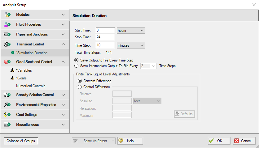
The XTS module is used to model the process demand changes over the 24-hour analysis period. Navigate to the Simulation Duration panel in the Transient Control group to view the Transient Control settings. Change the Start Time units to hours and enter a Stop Time of 24. For Time Step, changes the units to minutes and enter 10. The Simulation Duration panel should now look like Figure 4. The transient analysis is now set to run for a period of 24-hours with a time step of 10 minutes. Click OK to save and close Analysis Setup.
Step 7. Junction Transient Data
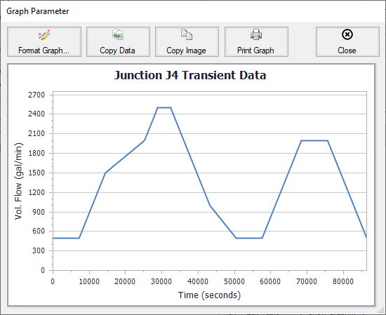
The flow variation in this model is driven by the J4 Assigned Flow junction. Open the J4 Assigned Flow Properties window and select the Transient tab. The process flow demands are modeled as time-varying flows. The flow profile over the 24-hour period is defined in the Transient Data table. Use Table 1 below to fill in the Transient Data table. Then, click Show Graph and make sure the Junction J4 Transient Data graph matches Figure 5.
Note that the time units are in seconds. Alternatively, you can change the preferred time units in User Options from seconds to hours to change the units of this table, then enter the values in this table in hours instead. However, to keep to the default units, this table is provided in time units of seconds.
Table 1: Transient Data table for J4 Assigned Flow
| Data Point | Time (seconds) | Vol. Flow (gal/min) |
|---|---|---|
| 1 | 0 | 500 |
| 2 | 7200 | 500 |
| 3 | 14400 | 1500 |
| 4 | 25200 | 2000 |
| 5 | 28800 | 2500 |
| 6 | 32400 | 2500 |
| 7 | 43200 | 1000 |
| 8 | 50400 | 500 |
| 9 | 57600 | 500 |
| 10 | 64800 | 1500 |
| 11 | 68400 | 2000 |
| 12 | 75600 | 2000 |
| 13 | 82800 | 1000 |
| 14 | 86400 | 500 |
In addition, the J3 Reservoir junction is modeled as a finite reservoir (Figure 6). The J3 Reservoir can potentially drain and fill, and the varying pump speed (and, hence, flow) is what will keep its liquid level at 15 feet. No further input is required for the Supply Tank.
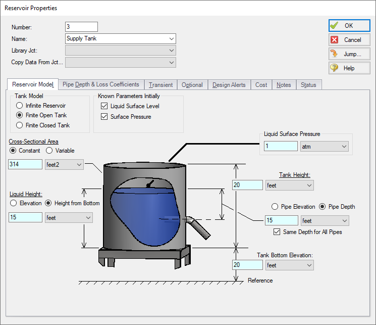
Figure 6: J3 Reservoir junction is finite, which means it can drain and fill
Step 8. Cost Settings
For this problem, the pump energy cost for the 24-hour analysis period is entered as a fixed energy cost on the Cost Settings panel. Open the Cost Settings panel from the Analysis Setup window to view the energy cost settings ().
For Cost Calculation, select Calculate. Under Cost Definitions, check the box for Operation/Energy because that is the only cost of interest for this example.
Set the Cost Time Period System Life to 1 year. The 24-hour operation is assumed to repeat every day for this one-year period, and the total energy cost will be calculated assuming the 24-hour operation repeats non-stop throughout the year. More complicated cost variation is possible when using energy cost libraries.
For Energy Cost, make sure Use This Energy Cost Information is selected and enter a Cost of 0.06 U.S. Dollars Per kW-hr.
The Cost Setting panel should now look like Figure 7 below.
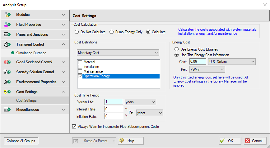
Figure 7: Cost Settings window applies Operation/Energy cost, can set the energy cost, and specifies the cost time period
Return to the Workspace and open the properties window for Pump J2. Navigate to the Cost tab and under Cost Report, select Include Cost in Report. Click OK.
Step 9. Run the Model
Click Run Model on the toolbar or from the Analysis menu. This will open the Solution Progress window. This window allows you to watch as the AFT Fathom solver converges on the answer. This model runs very quickly. Now view the results by clicking the Output button at the bottom of the Solution Progress window.
Note: When the GSC and XTS modules are used simultaneously, the GSC module is rerun for each time step. The GSC module variables are recalculated for the system conditions at each time step to ensure the specified goals are always met. This will typically result in longer run times, due to the increase in solution iterations that must be solved for each time step analysis.
Step 10. Examine the Output
When using multiple modules, the goal seek, transient and cost analysis results are shown in the Output window in the same manner as when they are used individually.
First open Output Control and go to the Format & Action tab. In the Time Simulation Formatting section, change the units to hours. Now all time units for XTS related output parameters will be shown using time units of hours.
The GSC variable and goal results in the General Output section can be viewed for each time step by using the slider bar at the bottom of the Output window, as shown in Figure 8.
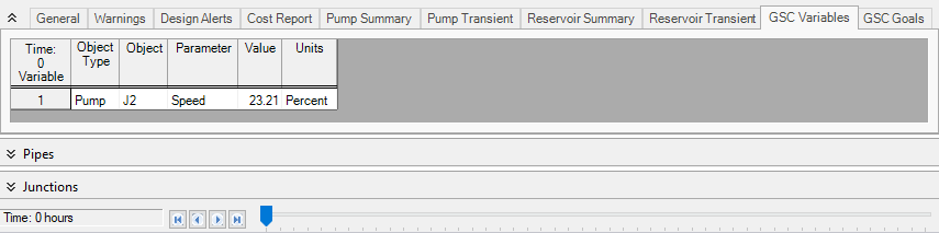
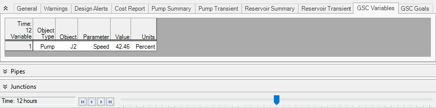
Figure 8: The slider bar at the bottom of the Output window can be used to view the transient results at any time step, including the GSC module variable and goal results. The GSC variable results for Time = 0 hours and Time = 12 hours are shown
Cost data is displayed in the Cost Report in the General Output section, as shown in Figure 9. The one-year energy cost for the supply pump in this example was
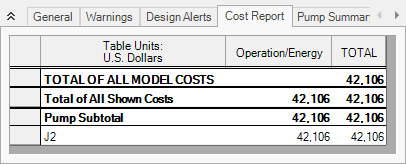
Figure 9: The cost data is shown in the Cost Report in the General Output section of the Output window
Figure 10 shows how the GSC module varied the pump's speed over time with the varying process flow rate. Figure 11 shows that the water level in the process supply tank remains constant over time (which was the goal). The pump speed changes to increase and decrease the flow in order to keep the net flow into the Supply Tank zero.
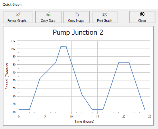
Figure 10: The GSC module varies the supply pump speed as the process flow rate changes over time (top)
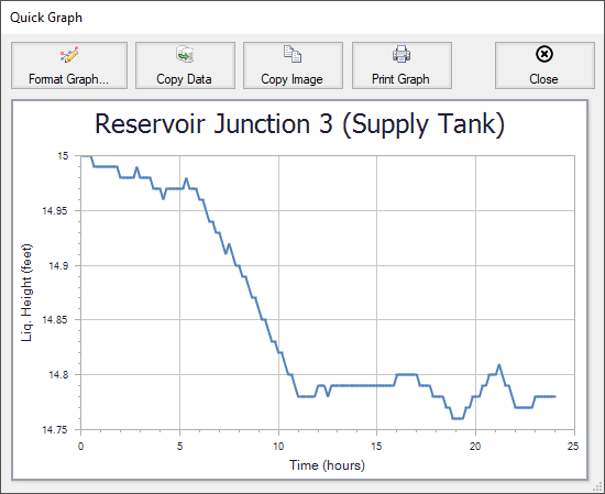
Figure 11: The water level in the process supply tank remains constant over time due to the variation in the pump speed (bottom)
Summary
Individually, the AFT Fathom modules provide you with powerful analytical tools to assist you in the design of your pipe systems. The ability to combine the capabilities of these tools provides you with even greater and more powerful modeling capabilities.


