Non-Newtonian Mill Discharge Slurry (English Units)
Non-Newtonian Mill Discharge Slurry (Metric Units)
Summary
This example demonstrates how one can take small-scale raw rheological data for a mill slurry at a minerals plant and use it on a full-scale pipe calculation.
Topics Covered
-
Reviewing and entering rheological data
-
Using homogeneous scale-up features
-
Obtaining and using Power Law and Bingham Plastic constants
Required Knowledge
This example assumes the user has already worked through the Beginner: Three Reservoir Problem example, or has a level of knowledge consistent with that topic. You can also watch the AFT Fathom Quick Start Video Tutorial Series on the AFT website, as it covers the majority of the topics discussed in the Three-Reservoir Problem example.
In addition the user should have worked through Non-Newtonian Phosphates Pumping example.
Model Files
This example uses the following files, which are installed in the Examples folder as part of the AFT Fathom installation:
Problem Statement
The piping for a non-settling slurry for a mill discharge at a minerals plant is being designed. The system will supply
Rheological data using the actual fluid in a 1/4 inch pipe has been obtained. Perform non-settling slurry calculations to evaluate how well the Bingham Plastic and Power Law models follow the raw data. Then determine the pressure drop in the full-scale pipe using Bingham Plastic, Power Law and Homogeneous Scale-up models.
Step 1. Review Raw Data in Excel
The data taken for 1/4 inch STD schedule (
Density =
Table 1: Pressure drop data on mill slurry (1/4 inch pipe -
| Run | Q (gal/min) | dP (psid) |
|---|---|---|
| 1 | 0.013 | 3.6 |
| 2 | 0.066 | 5.2 |
| 3 | 0.110 | 6.4 |
| 4 | 0.220 | 7.7 |
| 5 | 0.440 | 8.7 |
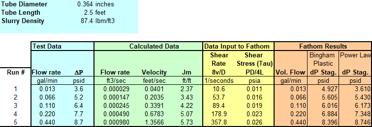
The Bingham Plastic and Power Law models typically process data in terms of shear rate and shear stress. The above data needs to be changed into a form for input into AFT Fathom.
Open the provided Excel spreadsheet Non-Newtonian Mill Discharge Slurry Data.xlsx. Click the Excel tab for
Step 2. Start AFT Fathom
From the Start Menu choose the AFT Fathom 12 folder and select AFT Fathom 12.
To ensure that your results are the same as those presented in this documentation, this example should be run using all default AFT Fathom settings, unless you are specifically instructed to do otherwise.
Step 3. Define the Fluid Properties Group
-
Open Analysis Setup from the toolbar or from the Analysis menu.
-
Open the Fluid panel:
-
Fluid Library = User Specified Fluid
-
Name = Mill Discharge Slurry
-
Density = 87.4 lbm/ft3
-
Dynamic Viscosity = 10 lbm/hr-ft (note that the viscosity entered here will not be used once the non-Newtonian parameters are entered)
-
-
Open the Viscosity Model panel
-
Viscosity Model = Bingham Plastic
-
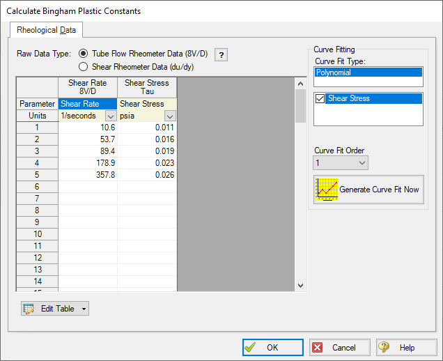
Select Calculate from Rheological Data
-
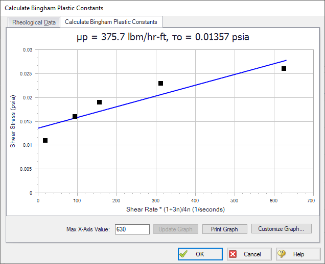
Click Calculate Constants
-
Raw Data Type = Tube Flow Rheometer Data (8V/D)
-
Raw Data =
-
| Parameter | Shear Rate | Shear Stress |
|---|---|---|
| Units | 1/seconds | psia |
| 1 | 10.6 | 0.011 |
| 2 | 53.7 | 0.016 |
| 3 | 89.4 | 0.019 |
| 4 | 178.9 | 0.023 |
| 5 | 357.8 | 0.026 |
-
Curve Fit Order = 1
Step 4. Define the Pipes and Junctions Group
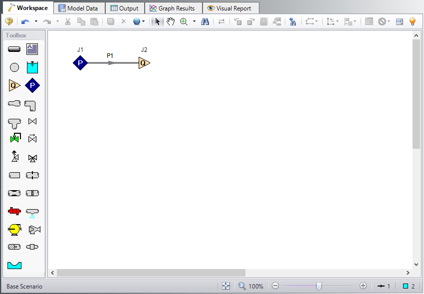
At this point, the first two groups are completed in Analysis Setup. The next undefined group is the Pipes and Junctions group. To define this group, the model needs to be assembled with all pipes and junctions fully defined. Click OK to save and exit Analysis Setup then assemble the model on the workspace as shown in the figure below.
Pipe Properties
-
Pipe Material = Steel - ANSI
-
Pipe Geometry = Cylindrical Pipe
-
Size = 1/4 inch
-
Type = STD (schedule 40)
-
Length = 2.5 feet
Junction Properties
-
J1 Assigned Pressure
-
Elevation = 0 feet
-
Pressure = 100 psia
-
Pressure Specification = Stagnation
-
-
J2 Assigned Flow
-
Elevation = 0 feet
-
Type = Outflow
-
Flow Specification = Volumetric Flow Rate
-
Flow Rate = 0.013 gal/min
-
ØTurn on Show Object Status from the View menu to verify if all data is entered. If so, the Pipes and Junctions group in Analysis Setup will have a check mark. If not, the uncompleted pipes or junctions will have their number shown in red. If this happens, go back to the uncompleted pipes or junctions and enter the missing data.
Step 5. Run the Model
Click Run Model on the toolbar or from the Analysis menu. This will open the Solution Progress window. This window allows you to watch as the AFT Fathom solver converges on the answer. This model runs very quickly. Now view the results by clicking the Output button at the bottom of the Solution Progress window.
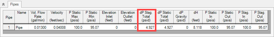
Step 6. Examine the Output
Figure 5 shows the Output window. It can be seen that the pressure drop is
Step 7. Create Scenarios
From the Base Scenario, make a child scenario named Bingham Plastic.
Step 8. Run Other Bingham Plastic Scenarios
Load the Bingham Plastic scenario and use the Duplicate Special feature to create five identical runs. Enter flow rates of
Step 9. Create and Run Power Law Scenarios
In the Scenario Manager, right click the Bingham Plastic scenario and select Clone Without Children. Name this scenario Power Law.
-
Load the Power Law Scenario
-
Open Analysis Setup
-
Open the Viscosity Model panel
-
Viscosity Model = Power Law
-
Select Calculate from Rheological Data
-
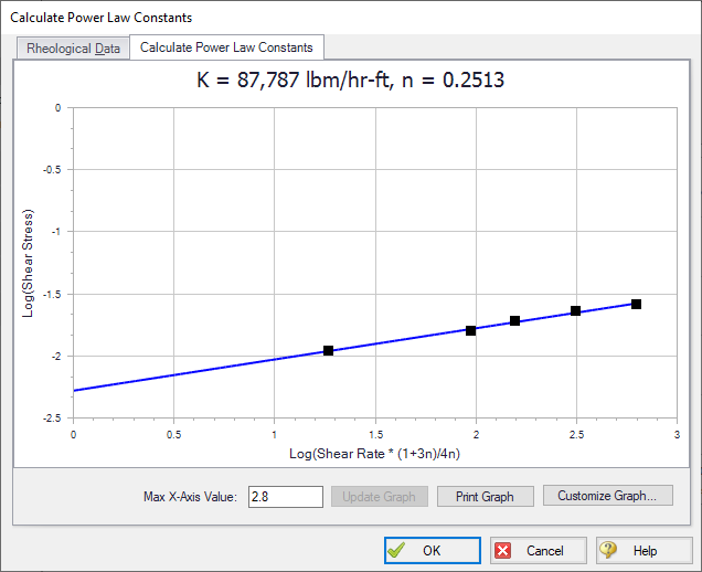
Click Calculate Constants
-
Raw Data Type = Tube Flow Rheometer Data (8V/D)
-
Raw Data = should still be loaded from before
-
Curve Fit Order = 1
-
Click Generate Curve Fit Now
-
Click OK
-
-
Click OK
Run the model again.
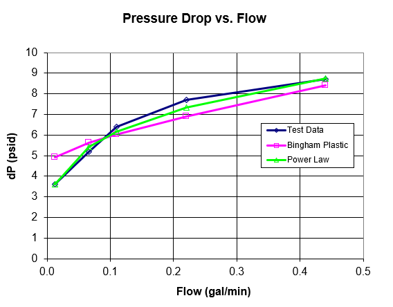
Figure 7 shows the output for each of the ten cases. Figure 8 plots the test data against the results of Bingham Plastic and Power Law. From Figure 8 it is clear the Power Law model fits the mill discharge slurry data better than Bingham Plastic.
Step 10. Evaluate Full Scale Data
-
Make another child scenario called Full Scale - 12 inch
-
Change pipe P1 to 300 feet length and 12 inch diameter
-
Change junction J2 to a flow rate of 880 gal/min
-
Make three child scenarios below Full Scale - 12 inch: one for each, Bingham Plastic, Power Law, and Homogeneous Scale-up
-
Load the Bingham Plastic scenario, open Analysis Setup, and perform a curve fit for Bingham Plastic
-
Run the Bingham Plastic scenario and note the pressure drop
-
Repeat the above for the Power Law scenario
-
For the Homogeneous Scale-up scenario, use the test data from the Excel spreadsheet. Make sure to enter the data as Volumetric in
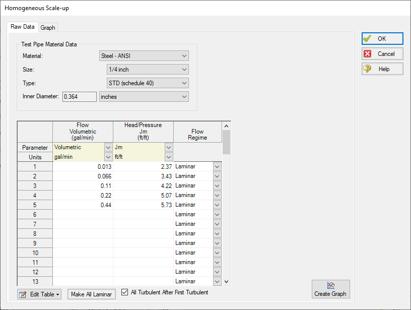
Figure 10 shows a comparison of pressure drop results using multi-scenario output for the three children. It can be seen that there is closer agreement between Power Law and Homogeneous Scale-up. The Bingham Plastic results are not as close which was true earlier in this example comparing to actual test data (Figure 8). Therefore the Bingham Plastic pressure drop should be excluded and the design pressure drop should be based on Power Law and Homogeneous Scale-up.
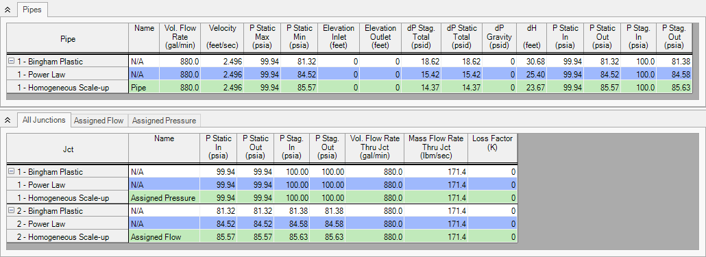
Figure 10: Full scale pressure drop comparison of Bingham Plastic, Power Law, and Homogeneous Scale-up
Analysis Summary
A non-settling mill discharge slurry for a minerals plant was modeled using non-settling slurry calculations in AFT Fathom. Runs for small scale and full-scale calculation were made and pressure drop was determined for these cases.


