Slurries with Variable Fluid Properties - SSL (English Units)
Slurries with Variable Fluid Properties - SSL (Metric Units)
Summary
This example demonstrates the fundamental concepts of the Settling Slurry (SSL) add-on module by way of example. The example shows how SSL can be used to model the introduction of solids into a clear fluid stream.
Evaluate pump and system performance for a slurry system that will pump 30% sand by volume for three cases:
-
Pumping clear water (no solids in system)
-
Solids introduced into the system, and propagated through to the pump discharge
-
Solids have propagated through the entire system
This example is essentially modeling four snapshots in time as the slurry is injected and pumped through the pipeline. These four snapshots in time can be modeled through the usage of the Volume Balance junction.
Note: This example can only be run if you have a license for the SSL module.
Topics Covered
-
Entering solids data
-
Using Volume Balance junctions with variable fluid properties
-
Creating slurry system curves and evaluating pump performance
Required Knowledge
This example assumes the user has already worked through the Walk-Through Examples section, and has a level of knowledge consistent with the topics covered there. If this is not the case, please review the Walk-Through Examples, beginning with the Beginner: Three Reservoir Model example. You can also watch the AFT Fathom Quick Start Video Tutorial Series on the AFT website, as it covers the majority of the topics discussed in the Three-Reservoir Model example.
In addition the user should have worked through Pump Sizing for Sand Transfer System - SSL example.
Model File
This example uses the following file, which is installed in the Examples folder as part of the AFT Fathom installation:
Step 1. Start AFT Fathom
From the Start Menu choose the AFT Fathom 12 folder and select AFT Fathom 12.
To ensure that your results are the same as those presented in this documentation, this example should be run using all default AFT Fathom settings, unless you are specifically instructed to do otherwise.
Step 2. Define the Modules Panel
Open Analysis Setup from the toolbar or from the Analysis menu. Navigate to the Modules panel. For this example, check the box next to Activate SSL and select Settling to enable the SSL module for use. The items in the Fluid Properties group will change to accommodate slurry definitions. Click OK to save the changes and exit Analysis Setup. Open the Analysis menu to see the new option called Slurry. From here you can quickly toggle between Disable mode (normal AFT Fathom) and Settling (SSL mode).
Step 3. Define the Fluid Properties Group
Open Analysis Setup from the toolbar or from the Analysis menu and input the following on the respective panels.
-
Carrier Fluid - Figure 1
-
Fluid Model = Advanced
-
Fluid Library = AFT Standard
-
Fluid = Water (liquid)
-
After selecting, click Add to Model
-
-
Temperature = 35 deg. F
-
Select Variable Fluid Properties
-
-
Solids Definition - Figure 2
-
Slurry Calculation Method = Simplified
-
Solids Specifications = User Specified Solids Added
-
M (Stratification Ratio Exponent) = User Specified
-
Value = 1.7
-
Density = 2.65 S.G. water
-
d50 = 0.016 inches
-
-
Slurry Definition - Figure 3
-
Slurry Calculation Method = Simplified (this selection will be the same as on the Solids Definition panel)
-
Concentration Type = Volume Fraction
-
Amount Solids Added = 30 Percent
-
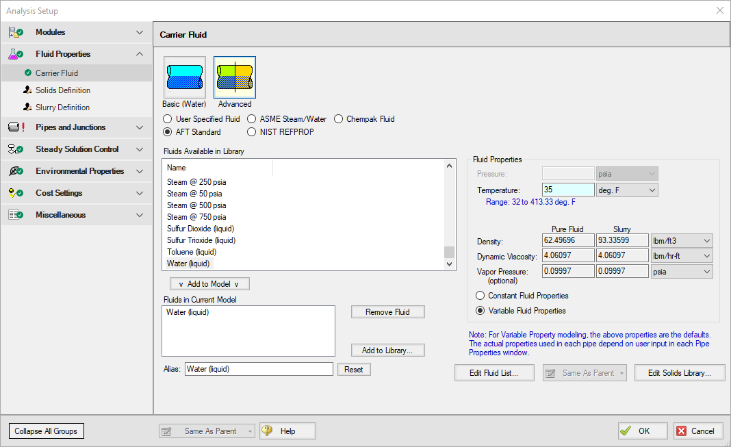
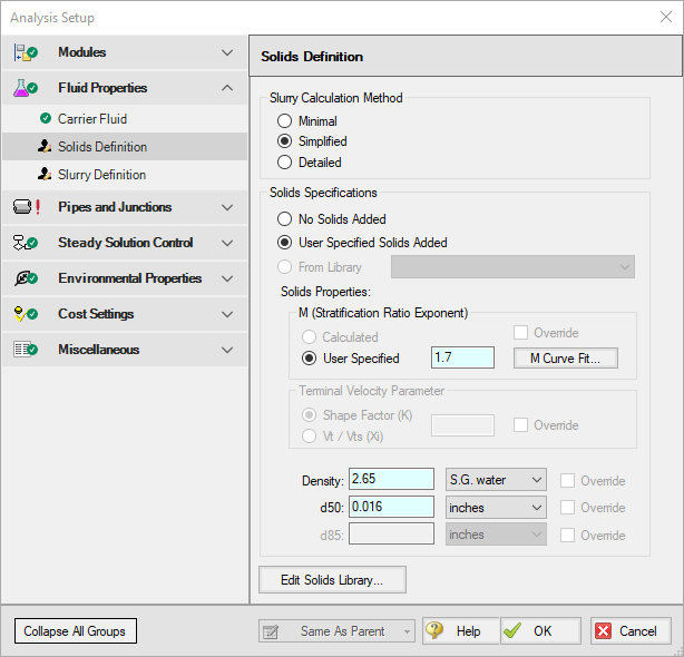
Figure 2: Solids Definition panel in the Fluid Properties group in Analysis Setup with SSL activated
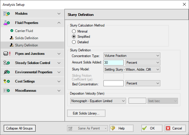
Figure 3: Slurry Definition panel in the Fluid Properties group in Analysis Setup with SSL activated
Step 4. Define the Pipes and Junctions Group
At this point, the first two groups are completed in Analysis Setup. The next undefined group is the Pipes and Junctions group. To define this group, the model needs to be assembled with all pipes and junctions fully defined. Click OK to save and exit Analysis Setup then assemble the model on the workspace as shown in the figure below.
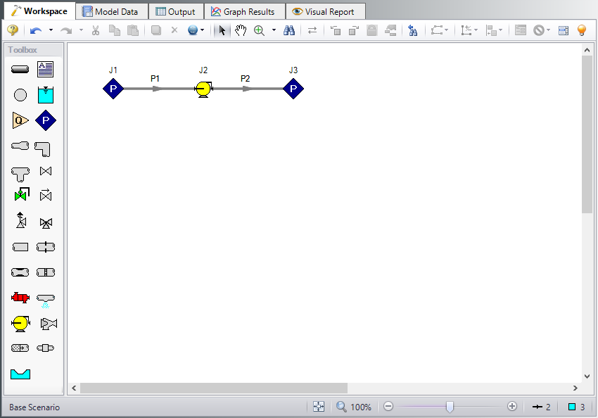
Enter the following pipe and junction properties.
Pipe Properties
-
All Pipes
-
Pipe Material = Steel - ANSI
-
Pipe Geometry = Cylindrical Pipe
-
Size = 6 inch
-
Type = STD (schedule 40)
-
Friction Model Data Set = Standard
-
Length =
| Pipe | Length (feet) |
|---|---|
| 1 | 50 |
| 2 | 1000 |
Junction Properties
-
J1 & J3 Assigned Pressures
-
Elevation = 0 feet
-
Pressure = 150 psig
-
Pressure Specification = Stagnation
-
-
J2 Pump
-
Inlet Elevation = 0 feet
-
Pump Model = Centrifugal (Rotodynamic)
-
Analysis Type = Pump Curve
-
Enter Curve Data =
-
| Volumetric | Head | Efficiency |
|---|---|---|
| gal/min | feet | Percent |
| 0 | 200 | - |
| 500 | 188 | 45 |
| 800 | 175 | 64 |
| 1100 | 155 | 75 |
| 1400 | 130 | 77 |
| 1700 | 100 | 74 |
-
Curve Fit Order = 2
ØTurn on Show Object Status from the View menu to verify if all data is entered. If so, the Pipes and Junctions group in Analysis Setup will have a check mark. If not, the uncompleted pipes or junctions will have their number shown in red. If this happens, go back to the uncompleted pipes or junctions and enter the missing data.
Step 5. Create the Scenarios
For this example, there are four cases to be examined. Create a scenario for each of the four cases, as shown in Figure 5:
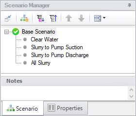
Clear Water Scenario
Load the Clear Water scenario by double-clicking the scenario name in the Scenario Manager.
This case requires that the pipes use clear water as their fluid. As pipes are drawn on the workspace, they automatically assume the same fluid type that is defined in the Analysis Setup window. As a result, at this point, all of the pipes are defined as using the sand slurry. Reset both pipes to use only water by opening the pipe properties window and inputting the following:
-
Fluid Properties tab
-
Fluid Properties button
-
In the Analysis Setup window that appears, click the Solids Definition item, and select No Solids Added, as shown in Figure 6. This will treat the fluid as clear water.
-
Click OK.
-
Make sure to do this to both pipes.
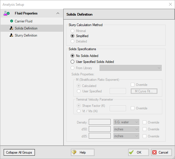
Figure 6: Fluids can be treated as clear fluid by selecting No Solids Added as the Solids Specification
Slurry to Pump Suction Scenario
Now load the Slurry to Pump Suction as the active scenario in the Workspace.
For the case where the fluid far upstream of the pump suction is slurry, and the fluid just upstream of the pump is clear water, a Volume Balance junction must be used to account for the difference in fluid density. The Volume Balance junction balances the flow based on volume rather than mass, ensuring that the velocity across the interface is the same. This junction must be used any time there is a system interface with fluids of different densities.
Add a Volume Balance junction just upstream of the pump suction by splitting the pipe as follows:
-
While holding the Shift key drag and drop the Volume Balance junction over pipe P1.
-
In the dialogue box set Pipe A as
-
Open the Volume Balance properties window for junction J4 and check that the elevation is 0
This case requires that the short pipe just upstream and the pipe downstream of the pump use clear water as their fluid. Set both pipes P2 and P3 to use only water as follows:
-
Fluid Properties tab
-
Fluid Properties button
-
In the Analysis Setup window that appears, click the Solids Definition item, and select No Solids Added, as shown in Figure 6. This will treat the fluid as clear water.
-
Click OK.
-
Make sure to do this to both pipes.
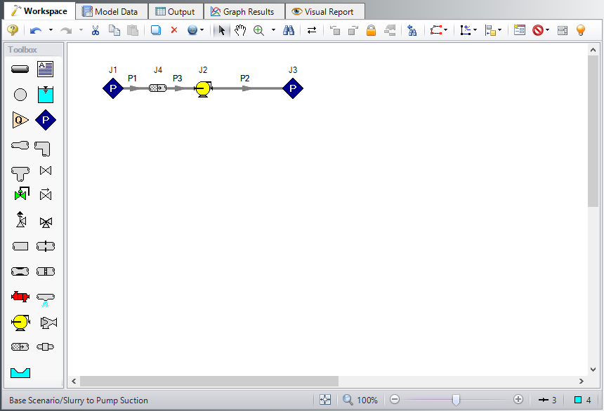
Figure 7: Layout of pipe system for partial slurry case with slurry at the pump suction showing the Volume Balance junction for the Slurries with Variable Fluid Properties example
Slurry to Pump Discharge Scenario
Load the Slurry to Pump Discharge scenario as the active scenario.
For the case where the fluid upstream and just downstream of the pump discharge is slurry, and the rest of the system downstream is clear water, a Volume Balance junction must be used again to account for the difference in fluid density.
Add a Volume Balance junction just downstream of the pump discharge by splitting pipe 2.
-
While holding the Shift key drag and drop the Volume Balance junction over pipe P2.
-
In the dialogue box set Pipe A as
-
Open the Volume Balance properties window for junction J5 and check that the elevation is 0
This case requires that the pipe P4 downstream of the pump use clear water as its fluid. Set pipe P4 to use only water as follows:
-
Fluid Properties tab
-
Fluid Properties button
-
In the Analysis Setup window that appears, click the Solids Definition item, and select No Solids Added, as shown in Figure 6. This will treat the fluid as clear water.
-
Click OK.
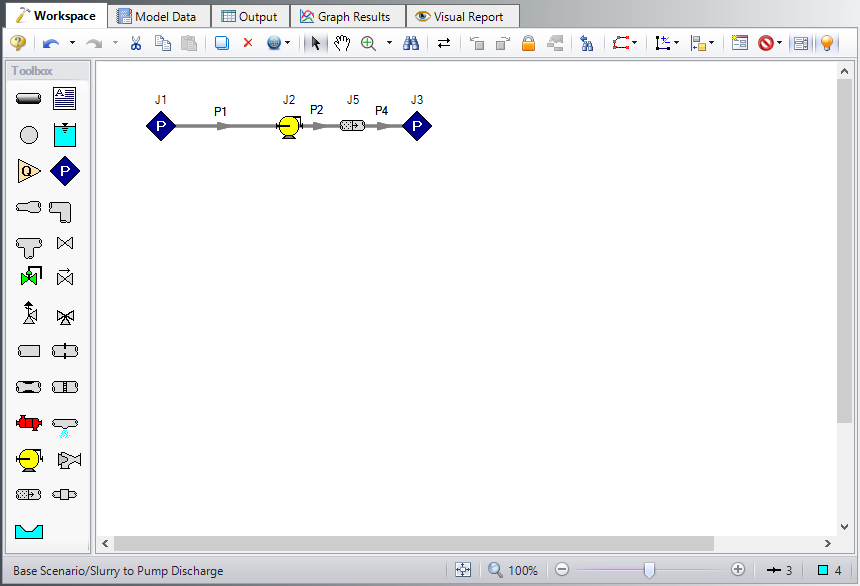
Figure 8: Layout of pipe system for partial slurry case with slurry at the pump discharge showing the Volume Balance junction for the Slurries with Variable Fluid Properties example
All Slurry Scenario
For this case, all of the pipes contain the sand slurry. The system layout is the same as is shown in Figure 4.
Step 6. Run the Model
Click Run Model on the toolbar or from the Analysis menu. This will open the Solution Progress window. This window allows you to watch as the AFT Fathom solver converges on the answer. This model runs very quickly. Now view the results by clicking the Output button at the bottom of the Solution Progress window.
Note: All scenarios can be run automatically by Fathom by completing a Batch Run from the File menu.
Step 7. Examine the Output
Table 1 shows the variation of the system flows, velocities, and pump performance as the slurry progresses through the system.
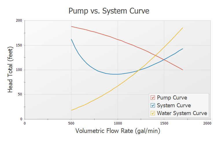
Figure 9 shows the pump curve plotted along with both the water and slurry system curves. This graph was generated in the All Slurry scenario using the Slurry System Curve graph type.
As the slurry progresses from the system inlet to the pump suction, the system volumetric flow rate, pump head, and power are not significantly changed (compare Table 1 output for Clear Water to Slurry to Pump Suction).
After the slurry arrives at the pump discharge (compare Table 1 output for Slurry to Pump Suction to Slurry to Pump Discharge), there is a notable increase in the system volumetric flow rate
Eventually the slurry fills the entire pipe (compare Table 1 output for Slurry to Pump Discharge to All Slurry). Because of the increased overall head loss of the slurry compared to water, the system shifts back on the pump curve to a lower flow rate
The power requirement on the pump increases from the Clear Water to All Slurry scenario as the system progresses from all water to all slurry.
Of significance here is the fact that, perhaps counter to intuition, the clear water and all slurry cases do not encompass the entire flow and system performance cases for the pump. The highest and lowest flow cases actually occur as the system is only partially full of slurry. Care should be taken to examine intermediate slurry flow cases to determine system feasibility for situations where slurry is being introduced into the flow, as the maximum and minimum flow cases will not necessarily occur when the system is flowing all clear fluid, or all slurry.
It is difficult to quantify the intermediate cases through the use of pump vs. system curves. This is a result of the variation in density that occurs in the system, which confuses the meaning of Head which itself depends on constant density. Thorough analysis is needed in these cases. Figure 9 shows the clear water and all slurry system curves.
Finally, note that to keep the example clearer, the effect of pump de-rating was not addressed. In real systems when the slurry progresses from the Slurry to Pump Suction case to the Slurry to Pump Discharge case, there will be a further decrease in pump performance which will effectively lower the pump curve in Figure 9. This would serve to shift operation to even higher flow rates for the Slurry to Pump Discharge and All Slurry cases.
Table 1: System flow and pump performance for different scenarios. The velocity and volumetric flow results are for the inlet of the pipe at the pump discharge
| Parameter | Vol. Flow Rate | Velocity | dP | dH | Overall Power |
|---|---|---|---|---|---|
| Units | gal/min | feet/sec | psid | feet | hp |
| Clear Water | 1,408 | 15.63 | 56.20 | 129.5 | 59.25 |
| Slurry to Pump Suction | 1,401 | 15.57 | 56.46 | 130.1 | 59.24 |
| Slurry to Pump Discharge | 1,594 | 17.70 | 72.09 | 111.2 | 88.21 |
| All Slurry | 1,497 | 16.63 | 78.42 | 121.0 | 88.54 |