Spray Discharge System (Metric Units)

Summary

The objective of this example is to find the minimum supply pressure needed to supply a system of eight spray discharge heads with at least 100 gal/min to each spray head. The system has one main supply line that branches into two supply lines that supply four sprayers each.

Topics Covered

• Using spray discharge junctions

• Iterating on a supply condition to reach a desired output condition

• Using Isometric Pipe Drawing Mode

Required Knowledge

This example assumes the user has already worked through the Beginner: Three Reservoir Problem example, or has a level of knowledge consistent with that topic. You can also watch the AFT Fathom Quick Start Video Tutorial Series on the AFT website, as it covers the majority of the topics discussed in the Three-Reservoir Problem example.

Model File

This example uses the following file, which is installed in the Examples folder as part of the AFT Fathom installation:

• US - Spray Discharge.fth

Step 1. Start AFT Fathom

From the Start Menu choose the AFT Fathom 12 folder and select AFT Fathom 12.

To ensure that your results are the same as those presented in this documentation, this example should be run using all default AFT Fathom settings, unless you are specifically instructed to do otherwise.

Step 2. Define the Fluid Properties Group

1. Open Analysis Setup from the toolbar or from the Analysis menu.

2. Open the Fluid panel then define the fluid:

   1. Fluid Library = AFT Standard

   2. Fluid = Water (liquid)

      1. After selecting, click Add to Model

   3. Temperature = 70 deg. F

Step 3. Define the Pipes and Junctions Group

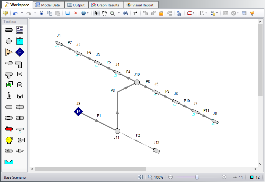
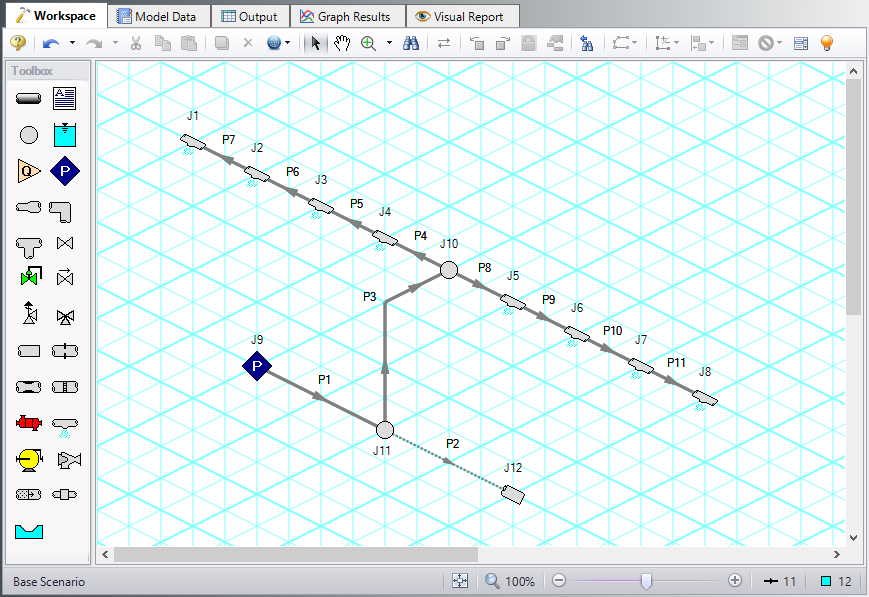
At this point, the first two groups are completed in Analysis Setup. The next undefined group is the Pipes and Junctions group. To define this group, the model needs to be assembled with all pipes and junctions fully defined. Click OK to save and exit Analysis Setup then assemble the model on the workspace as shown in the figure below.

The system is in place but now we need to enter the properties of the objects. Double-click each pipe and junction and enter the following properties. The required information is highlighted in blue.

Pipe Properties

1. Pipe Model tab

   1. Pipe Material = Steel - ANSI

   2. Pipe Geometry = Cylindrical Pipe

   3. Size = Use table below

   4. Type = STD (schedule 40)

   5. Friction Model Data Set = Standard

   6. Lengths =

Pipe	Size	Length (feet)
1 & 2	8 inch	500
3	4 inch	9
4 - 11	1-1/2 inch	10

Note: The Global Edit tool found in the Edit menu can be used to enter the data for pipes P4-P11 all at once. The Guide at the top right of the window can be used to walk you through how to global edit if needed.

Junction Properties

1. J1 - J8 Spray Discharges

   1. Elevation = 10 feet

   2. Loss Model = Cd Spray (Discharge Coefficient)

   3. Geometry = Spray Nozzle

   4. Exit Properties = Pressure

   5. Exit Pressure = 0 psig

   6. Cd (Discharge Coefficient) = 0.6

   7. Discharge Flow Area = 0.5 inches2

2. J9 Assigned Pressure

   1. Elevation = 1 feet

   2. Pressure = 200 psig

   3. Pressure Specification = Stagnation

3. J10 Branch

   1. Elevation = 10 feet

4. J11 Branch & J12 Dead End

   1. Elevation 1 feet

Note that the supply pressure is what we are trying to solve for, but we must supply a guess to start. We will need to iterate on the pressure at junction J9 to determine what the minimum pressure should be.

ØTurn on Show Object Status from the View menu to verify if all data is entered. If so, the Pipes and Junctions group in Analysis Setup will have a check mark. If not, the uncompleted pipes or junctions will have their number shown in red. If this happens, go back to the uncompleted pipes or junctions and enter the missing data.

Step 4. Run the Model

Click Run Model on the toolbar or from the Analysis menu. This will open the Solution Progress window. This window allows you to watch as the AFT Fathom solver converges on the answer. This model runs very quickly. Now view the results by clicking the Output button at the bottom of the Solution Progress window.

Step 5. Examine the Output

Open Output Control by selecting Output Control from the toolbar or Tools menu. Click the Junctions button, then add Vol. Flow Rate Net At Junction to the shown junction output. This output will show the volumetric flow rate discharged from the spray nozzle. Click OK to save the changes and close Output Control.

The Output window contains all the data that was specified in the Output Control window. In the Junction output window at the bottom of the page there is a special tab for Spray Discharge, as shown in Figure 2. Select this tab and examine the flow rate out of each of these junctions. All flow rates are above 100 gal/min so we must decrease the supply pressure and re-run the model. You should find that the supply pressure must be above 170.4 psig for the flow rate to meet the minimum flow rate at each spray nozzle.

This example may be solved directly using the GSC Module.

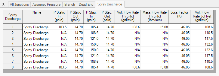
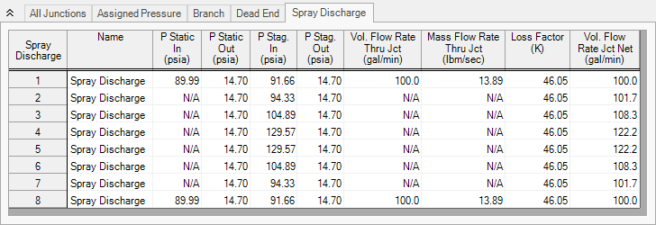
Figure 3 below displays the results for the final supply pressure of 170.4 psig.

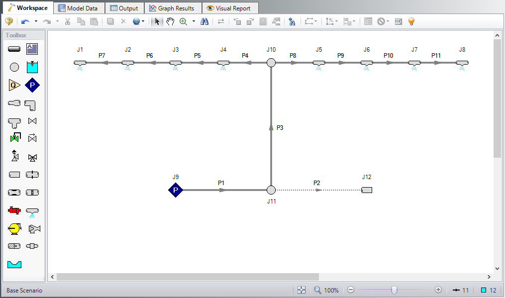
Step 6. Use the Isometric Grid

AFT Fathom allows the user to place pipe or junction objects anywhere in the Workspace. Objects are placed on a 2D grid by default, as was the case with this example. At times it may be convenient to demonstrate the three-dimensional nature of a system. For example, if you are building a model based on isometric reference drawings. AFT Fathom includes an isometric grid for these cases. The isometric grid has three gridlines that are offset by 60 degrees, representing the x, y, and z axes. Figure 4 shows the spray discharge system built on an isometric grid. The completed model file drawn in isometric can be seen in the Examples folder and is named Spray Discharge Isometric.

You can enable the isometric grid in AFT Fathom by going to the Arrange menu. Under Pipe Drawing Mode, there are three options: 2D Freeform (default), 2D Orthogonal, and Isometric.

Creating the spray discharge system on an isometric grid will demonstrate how to use this feature:

1. Go to the File menu and select New.

2. Go to the Arrange menu again and under Pipe Drawing Mode, select Isometric

3. Place a Spray Discharge junction, J1, on the Workspace. You will notice that placing junctions onto the Workspace follows the usual rules, however, the visual appearance of the icon is more complex than in a 2D grid. Due to the increased number of axes, the preferred icon and rotation must be selected to obtain visual consistency.

4. Right click on J1 and select Customize Icon. Select the icon shown in Figure 5.

Note: If a junction in isometric mode has at least two pipes connected to it, the Auto-rotate Icon option can be selected instead of Customize Icon. Auto-rotate icon will automatically choose the icon orientation based on the connected pipes.

5. Copy J1 for the other spray discharges, J2-J8, to maintain the preferred icon and rotation.

6. Place the assigned pressure junction, J9, on the Workspace.

7. Place two branch junctions, J10 and J11, on the Workspace.

8. Place the dead end junction, J12, on the Workspace.

9. Right click on J12 and select Customize Icon. Notice that you may need to use the Rotate button to get the preferred icon and rotation, as shown in Figure 6.

10. Draw Pipes 1 and 2, as shown in Figure 4.

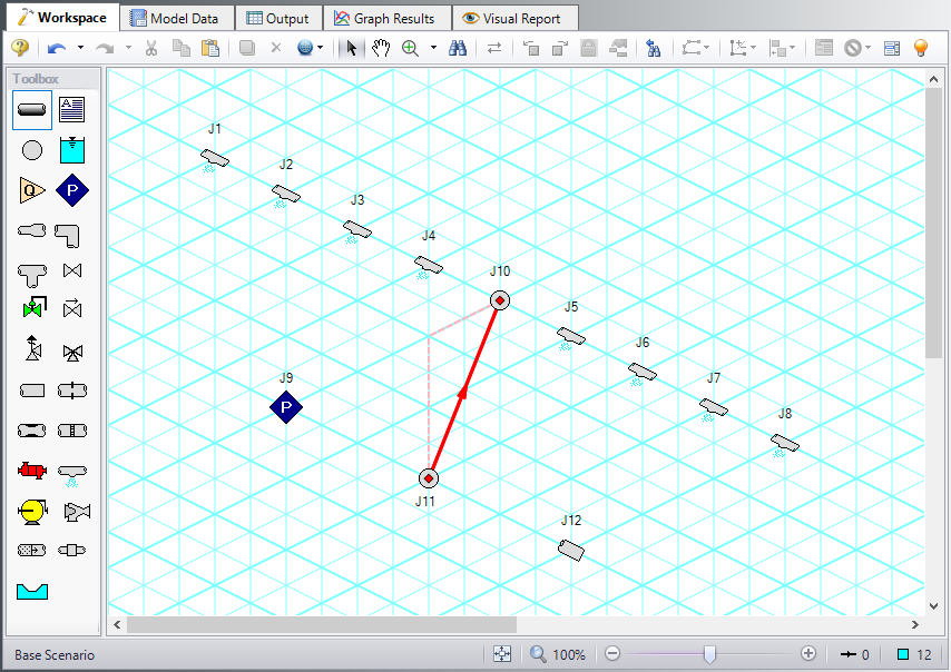
11. Draw Pipe 3 from J11 to J10. A red-dashed preview line will show how the pipe will be drawn on the isometric grid. As you are drawing a pipe, you can change the preview line by clicking any arrow key on your keyboard or scrolling the scroll wheel on your mouse.

Figure 7 shows Pipe 3 being drawn with the preview line.

Note: You can hold the ALT key while adjusting a pipe by the endpoint to add an additional vertex. This can be used with the arrow key or mouse scroll wheel to change between different preview line options.

12. Draw Pipes 4-11, as shown in Figure 4.

13. The grid can be shown or turned off in the Arrange menu. Figure 8 shows the completed model with the grid not shown.