Controlled Heat Exchanger Temperature - XTS (English Units)
Controlled Heat Exchanger Temperature - XTS (Metric Units)
Summary
Use the Extended Time Simulation module to determine the length of time required to fill the discharge reservoir, and to turn off the pump when the tank is full.
The discharge reservoir is a finite size tank,
Note: This example can only be run if you have a license for the XTS module.
Topics Covered
-
Defining Transient Control
-
Defining system transients
Required Knowledge
This example assumes the user has already worked through the Walk-Through Examples section, and has a level of knowledge consistent with the topics covered there. If this is not the case, please review the Walk-Through Examples, beginning with the Beginner: Three Reservoir Model example. You can also watch the AFT Fathom Quick Start Video Tutorial Series on the AFT website, as it covers the majority of the topics discussed in the Three-Reservoir Model example.
In addition, it is assumed that the user has worked through the Beginner: Filling a Tank - XTS example, and is familiar with the basics of XTS transient analysis.
Model Files
This example uses the following files, which are installed in the Examples folder as part of the AFT Fathom installation:
Step 1. Start AFT Fathom
From the Start Menu choose the AFT Fathom 12 folder and select AFT Fathom 12.
To ensure that your results are the same as those presented in this documentation, this example should be run using all default AFT Fathom settings, unless you are specifically instructed to do otherwise.
Step 2. Open the Model
Open the
Important: The XTS and GSC modules and cost calculations can be used in the same run to simulate control functions over time, but we are not going to do this here.
Step 3. Define the Modules Panel
Open Analysis Setup from the toolbar or from the Analysis menu. Navigate to the Modules panel. For this example, check the box next to Activate XTS and select Transient to enable the XTS module for use. A new group will appear in Analysis Setup titled Transient Control. Click OK to save the changes and exit Analysis Setup. Open the Analysis menu to see the new option called Time Simulation. From here you can quickly toggle between Steady Only mode (normal AFT Fathom) and Transient (XTS mode).
Note: The XTS module does not perform heat transfer calculations. You will be prompted to disable heat transfer calculations in order to proceed with modeling a transient. Click Yes.
Step 4. Define the Cost Settings group
Cost Calculation is not needed for this example. Go to the Cost Settings panel and select Do Not Calculate in the Cost Calculation section.
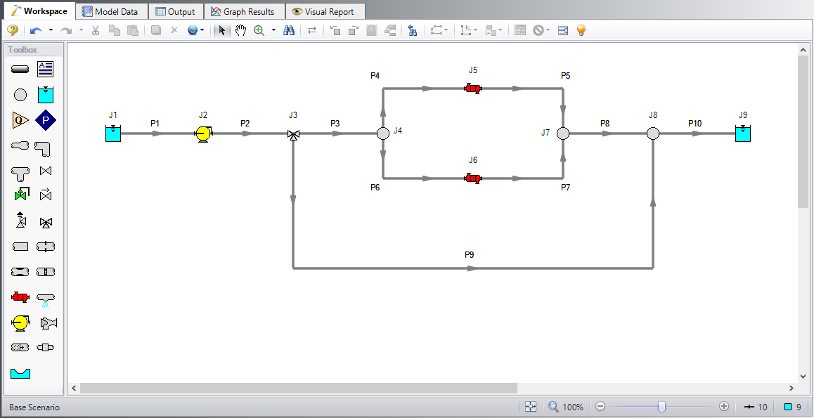
Step 5. Define Pipes and Junctions group
Most of the input is already entered. The only exception is for Reservoir J9. Enter the following junction properties.
-
J3 Three Way Valve
-
Library Jct = (None)
-
Actual Percent Open = 86 %
-
This value comes from the Actual Percent Open value calculated from the GSC example
-
-
J9 Reservoir
-
Name = Discharge Reservoir
-
Tank Model = Finite Open Tank
-
Known Parameters Initially = Liquid Surface Level & Surface Pressure
-
Cross-Sectional Area = Constant, 80 feet2
-
Liquid Level Specification = Height from Bottom
-
Liquid Height = 0 feet
-
Liquid Surface Pressure = 40 psig
-
Tank Height = 20 feet
-
Pipe Elevation = 10 feet
-
Tank Bottom Elevation = 10 feet
-
Step 6. Setup the Transient Data
For this example, we will set an event-based transient on the pump so the pump will turn off when the liquid level in the discharge tank reaches
You will define a single transient event. The event will occur when the liquid height in the reservoir reaches
Open the Pump Properties window, and enter the following information. Then the Transient tab should appear as shown in Figure 2.
-
Library Jct = (None)
-
Transient tab
-
Transient Type = Speed vs. Time
-
Transient Special Condition = None
-
Initiation of Transient = Single Event
-
Event Type = Reservoir Liquid Height
-
Condition = Greater Than or Equal To
-
Value = 20 feet
-
Junction = 9 (Discharge Reservoir)
-
Transient Data = Absolute Values
-
Data Points =
-
| Time (seconds) | Speed (Percent) |
|---|---|
| 0 | 100 |
| 10 | 0 |
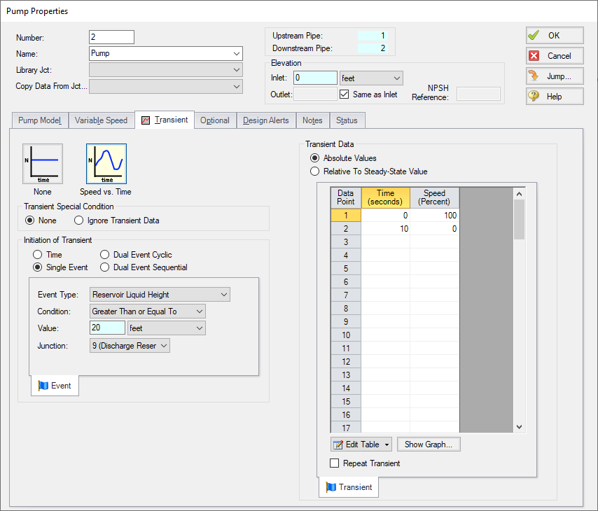
Figure 2: Junction transients are specified on the Transient tabs on the junction Properties windows
ØTurn on Show Object Status from the View menu to verify if all data is entered. If so, the Pipes and Junctions group in Analysis Setup will have a check mark. If not, the uncompleted pipes or junctions will have their number shown in red. If this happens, go back to the uncompleted pipes or junctions and enter the missing data.
Step 7. Define the Transient Control Group
Open Analysis Setup again and navigate to the Simulation Duration panel, part of the Transient Control group.
For this example, with a Start Time of 0 minutes, set the Stop Time to 45 minutes with a time step of 1 minute. The output will be saved to the output file for every time step.
Step 8. Specify the Time Simulation Formatting
Open the Output Control window and select the Format & Action tab. Set the Time Simulation Formatting units to minutes and click OK to save and close the window.
Step 9. Run the Model
Click Run Model on the toolbar or from the Analysis menu. This will open the Solution Progress window. This window allows you to watch as the AFT Fathom solver converges on the answer. This model runs very quickly. Now view the results by clicking the Output button at the bottom of the Solution Progress window.
Step 10. Examine the Output
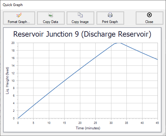
The transient reservoir data shows that the water in the discharge tank reached a height of
The Quick Graph plot (Figure 3) shows the tank liquid height over time. To create this graph, go to the Reservoir Transient tab in the top section of the window, then right-click on any of the Liq. Height cells for the Discharge Reservoir, junction J9, and select the Quick Graph option. There is an increase in the tank liquid height until the time when the pump turns off. The graph then shows that there is actually back flow into the system, due to the hydrostatic pressure of the fluid in the tank. This explains why there is a Critical Warning, which states that the pump head cannot be predicted due to reverse flow through the pump. A check valve would need to be added to the system to prevent this situation in the case of pump shutdown.