Housing Project - XTS (Metric Units)

Summary

This example uses the XTS module to simulate a supply pump used to replenish a water storage tank that is used to supply water to a housing development. There is a requirement that the height of the liquid in the water supply tank is not to drop below 10 feet. Use the flow conditions specified in the 4 inch Pipe scenario (not the fire flow scenarios) of the Housing Project walk-through example as the basis for this example.

Note: This example can only be run if you have a license for the XTS module.

Topics Covered

• Using Dual Cyclic Junction Transients

• Understanding Transient Output

• Resolving Time Step issues

Required Knowledge

This example assumes the user has already worked through the Walk-Through Examples section, and has a level of knowledge consistent with the topics covered there. If this is not the case, please review the Walk-Through Examples, beginning with the Beginner: Three Reservoir Model example. You can also watch the AFT Fathom Quick Start Video Tutorial Series on the AFT website, as it covers the majority of the topics discussed in the Three-Reservoir Model example.

In addition, it is assumed that the user has worked through the Beginner: Filling a Tank - XTS example, and is familiar with the basics of XTS transient analysis.

Model Files

This example uses the following files, which are installed in the Examples folder as part of the AFT Fathom installation:

• US - Housing Project.fth

• US - Housing Project - XTS.fth

Step 1. Start AFT Fathom

From the Start Menu choose the AFT Fathom 12 folder and select AFT Fathom 12.

To ensure that your results are the same as those presented in this documentation, this example should be run using all default AFT Fathom settings, unless you are specifically instructed to do otherwise.

Step 2. Open the model

Open the US - Housing Project.fth example file. Right-click on the 4 inch Pipe scenario and select Save Scenario to File Without Children and save this scenario to a new model file.

The Workspace should look like Figure 1 below:

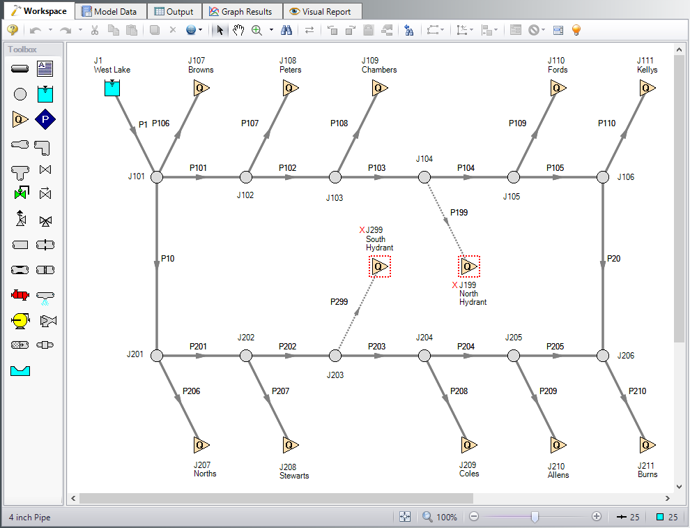
For this example, we will be changing the West Lake junction (J1) from an infinite reservoir to a finite water supply tank. We will then add a new supply reservoir, as well as a supply pump and a check valve to the system. The new supply pump will replenish the supply tank as the water level in the tank is depleted.

Step 3. Define the Modules Panel

Open Analysis Setup from the toolbar or from the Analysis menu. Navigate to the Modules panel. For this example, check the box next to Activate XTS and select Transient to enable the XTS module for use. A new group will appear in Analysis Setup titled Transient Control. Click OK to save the changes and exit Analysis Setup. Open the Analysis menu to see the new option called Time Simulation. From here you can quickly toggle between Steady Only mode (normal AFT Fathom) and Transient (XTS mode).

Step 4. Modify the existing model

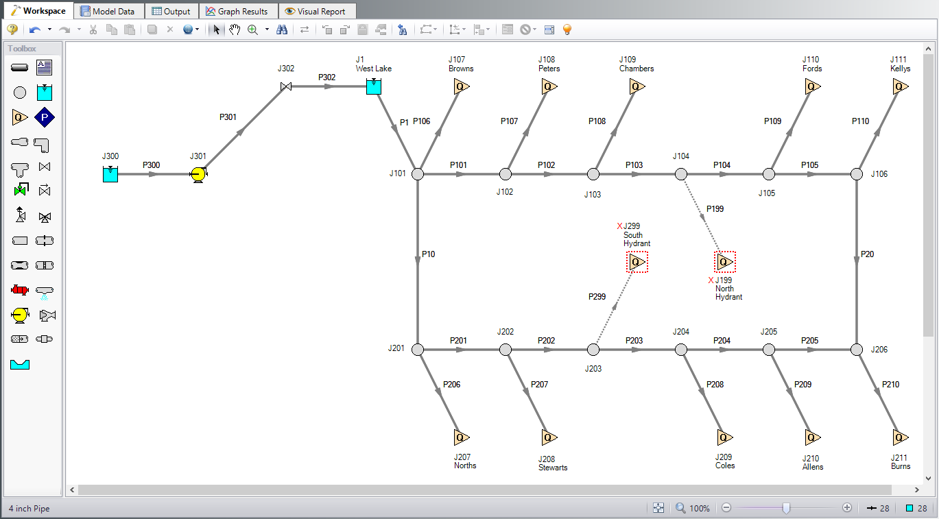
Modify the workspace to include the new supply reservoir, supply pump, check valve, and piping as shown in Figure 2. You may need to move the objects to the right on the Workspace to create room for the new pipes and junctions. Do this by selecting all pipes and junctions by either using CTRL+A or click-and-drag and selection box encompassing all objects. Then click, hold, and drag the objects to the right. Now define the new objects.

Pipe Properties

1. Pipe Model tab

   1. Pipe Material = PVC - ASTM

   2. Pipe Geometry = Cylindrical Pipe

   3. Size = 4 inch

   4. Type = schedule 40

   5. Friction Model Data Set = Standard

   6. Lengths =

Pipe	Length (feet)
300	25
301	500
302	5

Junction Properties

1. J300 Reservoir

   1. Name = West Lake

   2. Tank Model = Infinite Reservoir

   3. Liquid Surface Elevation = 0 feet

   4. Liquid Surface Pressure = 0 psig

   5. Pipe Depth = 0 feet

2. J301 Pump

   1. Inlet Elevation = 0 feet

   2. Pump Model = Centrifugal (Rotodynamic)

      1. Analysis Type = Pump Curve

      2. Enter Curve Data =

Volumetric	Head
gal/min	feet
0	1000
200	1150
400	800

3. Curve Fit Order = 2

3. Optional tab

   1. Special Condition = Pump Off With Flow Through

1. J302 Check Valve

   1. Inlet Elevation = 200 feet

   2. Loss Model = Cv

   3. Cv = 10

   4. Forward Velocity to Close Valve = 0 feet/sec

   5. Delta Pressure/Head to Reopen = Pressure

   6. Delta Pressure = 0 psid

2. J1 Reservoir

   1. Name = Supply Tank

   2. Tank Model = Finite Open Tank

   3. Known Parameters Initially = Liquid Surface Level & Surface Pressure

   4. Cross-Sectional Area = Constant, 80 feet2

   5. Liquid Level Specification = Height from Bottom

   6. Liquid Height = 15 feet

   7. Liquid Surface Pressure = 0 psig

   8. Tank Height = 15 feet

   9. Pipe Depth = 15 feet

   10. Tank Bottom Elevation = 200 feet

Step 5. Define the Transient Control Group

Open Analysis Setup again and navigate to the Simulation Duration panel, part of the Transient Control group.

For this example, with a Start Time of 0 minutes, set the Stop Time to 120 minutes with a time step of 1 minute. The output will be saved to the output file for every time step.

Step 6. Specify the Time Simulation Formatting

Open the Output Control window and select the Format & Action tab. Set the Time Simulation Formatting units to minutes and click OK to save and close the window.

Step 7. Enter the Pump Transient Data

For this example, the pump will be set to turn on when the liquid level in the supply tank drops below 10 feet, and turn off when the water level returns to 15 feet. To do this, we will use a Dual Event Cyclic event transient.

The Dual Event Cyclic event requires that two transients be defined. In this case, the first transient will be the pump turning on when the water level drops below 10 feet, and the second transient will be the pump turning off when the water level returns to 15 feet. The pump speed transients need to be included for both transient events as well. Enter the following in the pump properties window.

1. Transient tab

   1. Transient Type = Speed vs. Time

   2. Transient Special Condition = None

   3. Initiation of Transient = Dual Event Cyclic

   4. First Event

      1. Event Type = Reservoir Liquid Height

      2. Condition = Less Than or Equal To

      3. Value = 10 feet

      4. Junction = 1 (Supply Tank)

   5. First Transient =

Time (seconds)	Speed (Percent)
0	0
30	100

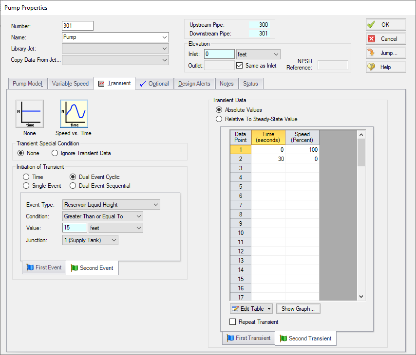
5. Second Event

   1. Event Type = Reservoir Liquid Height

   2. Condition = Greater Than or Equal To

   3. Value = 15 feet

   4. Junction = 1 (Supply Tank)

5. Second Transient =

Time (seconds)	Speed (Percent)
0	100
30	0

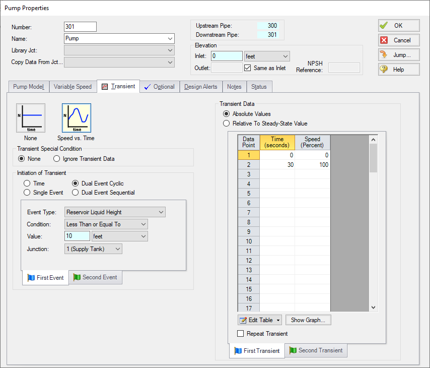
For this example, at the beginning of the simulation, the storage tank is full, so the pump will not be running initially. To account for this, the pump Special Condition on the Optional Tab must be set to Pump Off With Flow Through. In order to be consistent, the First Transient defined must be defined with an initial speed of 0, indicating a pump startup.

ØTurn on Show Object Status from the View menu to verify if all data is entered. If so, the Pipes and Junctions group in Analysis Setup will have a check mark. If not, the uncompleted pipes or junctions will have their number shown in red. If this happens, go back to the uncompleted pipes or junctions and enter the missing data.

Step 8. Run the Model

Click Run Model on the toolbar or from the Analysis menu. This will open the Solution Progress window. This window allows you to watch as the AFT Fathom solver converges on the answer. This model runs very quickly. Now view the results by clicking the Output button at the bottom of the Solution Progress window.

Step 9. Examine the Output

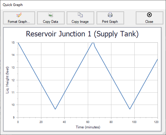
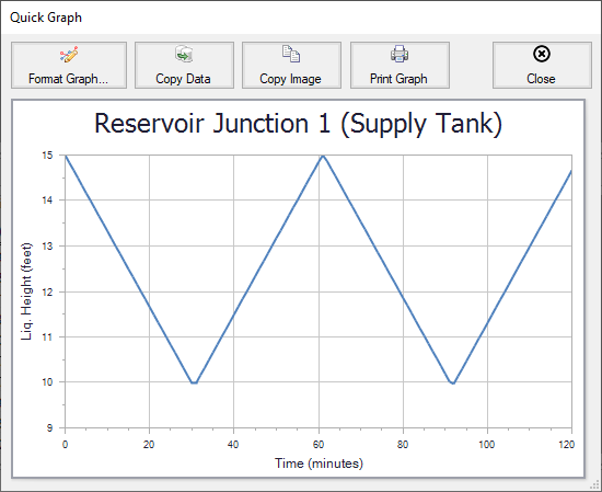
Figure 5 shows a Quick Graph plot of the liquid height in the J1 Supply Tank. The plot illustrates how the Dual Event Cyclic transient will repeat continuously as the event to trigger each transient is met, in turn. The plot shows the tank draining due to the flow to the housing project. When the liquid level reaches 10 feet, the pump starts, causing the liquid level in the tank to rise again. When the level reaches 15 feet, the transient to stop the pump is initiated. The tank begins to drain, until the level drops to 10 feet, and the pump is started again.

The plot shows the liquid level dropping below 10 feet. This is due, primarily with the time step resolution that was set in Transient Control. The time step was set to 1 minute, but the pump startup transient is 30 seconds. The size of the time step leads to overshoot in the calculations. Open the Simulation Duration panel, and set the time step to 10 seconds. Set the output to save to file every 6th time step (write output once every minute). The results from this case are shown in Figure 6. The results using the 10-second time step clearly show the effect of using the smaller time step.

The user should always carefully consider the time step being used in relation to the length of the transient events defined for their analysis.

Note: You may notice a warning message indicating that the static pressure is lower than vapor pressure at the outlet of pipe 301. Since this example is for demonstration purposes only, this warning may be ignored. However, warnings should othersie never be ignored.