Reservoir Balance - XTS (English Units)
Reservoir Balance - XTS (Metric Units)
Summary
The objective of this example is to demonstrate how the interaction of different hydrostatic pressures between can be analyzed using the XTS module. This example will use three finite reservoirs connected in series, with different initial liquid elevations.
Note: This example can only be run if you have a license for the XTS module.
Topics Covered
-
Using Finite Reservoirs Junctions
Required Knowledge
This example assumes the user has already worked through the Walk-Through Examples section, and has a level of knowledge consistent with the topics covered there. If this is not the case, please review the Walk-Through Examples, beginning with the Beginner: Three Reservoir Model example. You can also watch the AFT Fathom Quick Start Video Tutorial Series on the AFT website, as it covers the majority of the topics discussed in the Three-Reservoir Model example.
In addition, it is assumed that the user has worked through the Beginner: Filling a Tank - XTS example, and is familiar with the basics of XTS transient analysis.
Model File
This example uses the following file, which is installed in the Examples folder as part of the AFT Fathom installation:
Step 1. Start AFT Fathom
From the Start Menu choose the AFT Fathom 12 folder and select AFT Fathom 12.
To ensure that your results are the same as those presented in this documentation, this example should be run using all default AFT Fathom settings, unless you are specifically instructed to do otherwise.
Step 2. Define the Modules Panel
Open Analysis Setup from the toolbar or from the Analysis menu. Navigate to the Modules panel. For this example, check the box next to Activate XTS and select Transient to enable the XTS module for use. A new group will appear in Analysis Setup titled Transient Control. Click OK to save the changes and exit Analysis Setup. Open the Analysis menu to see the new option called Time Simulation. From here you can quickly toggle between Steady Only mode (normal AFT Fathom) and Transient (XTS mode).
Step 3. Define the Fluid Properties Group
-
Open Analysis Setup from the toolbar or from the Analysis menu.
-
Open the Fluid panel then define the fluid:
-
Fluid Library = AFT Standard
-
Fluid = Water (liquid)
-
After selecting, click Add to Model
-
-
Temperature = 70 deg. F
-
Step 4. Define the Pipes and Junctions Group
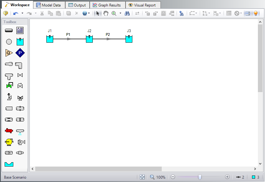
At this point, the first two groups are completed in Analysis Setup. The next undefined group is the Pipes and Junctions group. To define this group, the model needs to be assembled with all pipes and junctions fully defined. Click OK to save and exit Analysis Setup then assemble the model on the workspace as shown in the figure below.
Pipe Properties
Enter the following for both pipes P1 and P2.
-
Pipe Model tab
-
Pipe Material = Steel - ANSI
-
Pipe Geometry = Cylindrical Pipe
-
Size = 4 inch
-
Type = STD (schedule 40)
-
Friction Model Data Set = Standard
-
Length = 250 feet
-
Junction Properties
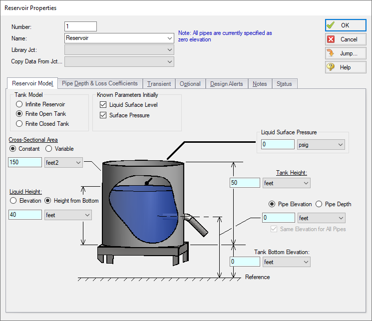
Figure 2 shows the Reservoir Properties window for junction J1. In the Fathom XTS module, reservoir junctions can have finite dimensions. The reservoirs can also be open, or closed. If the tank is closed, the user must specify the gas thermodynamics inside the closed tank. Users may also specify different initial known parameters for the reservoir. If only the Liquid Surface level is known, Fathom will calculate the Surface Pressure. Alternatively, if only the Surface Pressure is known, Fathom will calculate the Liquid Height. When using a reservoir as a finite tank, users must also specify the tank height, the initial liquid height in the tank, as well as the tank cross sectional area.
Next, define the reservoir junctions.
-
J1 Reservoir
-
Tank Model = Finite Open Tank
-
Known Parameters Initially = Liquid Surface Level & Surface Pressure
-
Cross-Sectional Area = Constant, 150 feet2
-
Liquid Level Specification = Height from Bottom
-
Liquid Height = 40 feet
-
Liquid Surface Pressure = 0 psig
-
Tank Height = 50 feet
-
Pipe Elevation = 0 feet
-
Tank Bottom Elevation = 0 feet
-
-
J2 Reservoir
-
Tank Model = Finite Open Tank
-
Known Parameters Initially = Liquid Surface Level & Surface Pressure
-
Cross-Sectional Area = Constant, 150 feet2
-
Liquid Level Specification = Height from Bottom
-
Liquid Height = 0 feet
-
Liquid Surface Pressure = 0 psig
-
Tank Height = 50 feet
-
Pipe Elevation = 0 feet
-
Tank Bottom Elevation = 0 feet
-
-
J3 Reservoir
-
Tank Model = Finite Open Tank
-
Known Parameters Initially = Liquid Surface Level & Surface Pressure
-
Cross-Sectional Area = Constant, 150 feet2
-
Liquid Level Specification = Height from Bottom
-
Liquid Height = 10 feet
-
Liquid Surface Pressure = 0 psig
-
Tank Height = 50 feet
-
Pipe Elevation = 0 feet
-
Tank Bottom Elevation = 0 feet
-
Step 5. Define the Transient Control Group
Open Analysis Setup again and navigate to the Simulation Duration panel, part of the Transient Control group.
For this example, with a Start Time of 0 minutes, set the Stop Time to 120 minutes with a time step of 1 minute. The output will be saved to the output file for every time step.
Step 6. Specify the Time Simulation Formatting
Open the Output Control window and select the Format & Action tab. Set the Time Simulation Formatting units to minutes and click OK to save and close the window.
ØTurn on Show Object Status from the View menu to verify if all data is entered. If so, the Pipes and Junctions group in Analysis Setup will have a check mark. If not, the uncompleted pipes or junctions will have their number shown in red. If this happens, go back to the uncompleted pipes or junctions and enter the missing data.
Step 7. Run the Model
Click Run Model on the toolbar or from the Analysis menu. This will open the Solution Progress window. This window allows you to watch as the AFT Fathom solver converges on the answer. This model runs very quickly. Now view the results by clicking the Output button at the bottom of the Solution Progress window.
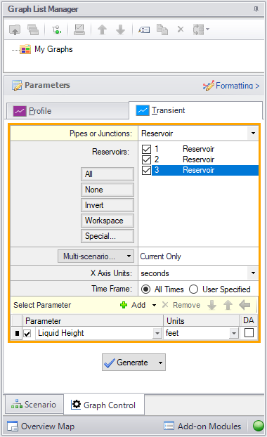
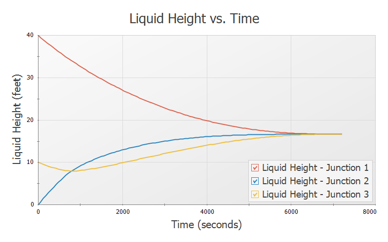
Step 8. Examine the Output
For this model, the output will be easiest to view as a graph, so select the Graph Results tab. Use the Graph Results window to plot the liquid height in each of the three reservoirs on the same plot. Figure 3 shows the Graph Control tab of the Quick Access Panel for simultaneously plotting the transient liquid height in all three reservoirs. Figure 4 show the resulting graph. Note that, as one would expect because the tanks are the same sizes and at the same elevations, the liquid heights between the tanks eventually reach the same equilibrium value.