Valve Closing - XTS (English Units)
Valve Closing - XTS (Metric Units)
Summary
The objective of this example is to demonstrate how to set up an event based transient in the XTS module for a valve junction. A valve is set to close when the liquid height in discharge tank reaches a specified level.
Note: This example can only be run if you have a license for the XTS module.
Topics Covered
-
Defining Junction Transients
-
Understanding Transient Output
Required Knowledge
This example assumes the user has already worked through the Walk-Through Examples section, and has a level of knowledge consistent with the topics covered there. If this is not the case, please review the Walk-Through Examples, beginning with the Beginner: Three Reservoir Model example. You can also watch the AFT Fathom Quick Start Video Tutorial Series on the AFT website, as it covers the majority of the topics discussed in the Three-Reservoir Model example.
In addition, it is assumed that the user has worked through the Beginner: Filling a Tank - XTS example, and is familiar with the basics of XTS transient analysis.
Model File
This example uses the following file, which is installed in the Examples folder as part of the AFT Fathom installation:
Step 1. Start AFT Fathom
From the Start Menu choose the AFT Fathom 12 folder and select AFT Fathom 12.
To ensure that your results are the same as those presented in this documentation, this example should be run using all default AFT Fathom settings, unless you are specifically instructed to do otherwise.
Step 2. Define the Modules Panel
Open Analysis Setup from the toolbar or from the Analysis menu. Navigate to the Modules panel. For this example, check the box next to Activate XTS and select Transient to enable the XTS module for use. A new group will appear in Analysis Setup titled Transient Control. Click OK to save the changes and exit Analysis Setup. Open the Analysis menu to see the new option called Time Simulation. From here you can quickly toggle between Steady Only mode (normal AFT Fathom) and Transient (XTS mode).
Step 3. Define the Fluid Properties Group
-
Open Analysis Setup from the toolbar or from the Analysis menu.
-
Open the Fluid panel then define the fluid:
-
Fluid Library = AFT Standard
-
Fluid = Water (liquid)
-
After selecting, click Add to Model
-
-
Temperature = 70 deg. F
-
Step 4. Define the Pipes and Junctions Group
At this point, the first two groups are completed in Analysis Setup. The next undefined group is the Pipes and Junctions group. To define this group, the model needs to be assembled with all pipes and junctions fully defined. Click OK to save and exit Analysis Setup then assemble the model on the workspace as shown in the figure below.
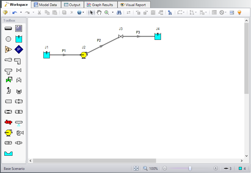
The system is in place but now we need to enter the properties of the objects. Double-click each pipe and junction and enter the following properties. The required information is highlighted in blue.
Pipe Properties
-
Pipe Model tab
-
Pipe Material = Steel - ANSI
-
Pipe Geometry = Cylindrical Pipe
-
Size = 4 inch
-
Type = STD (schedule 40)
-
Friction Model Data Set = Standard
-
Lengths =
-
| Pipe | Length (feet) |
|---|---|
| 1 | 10 |
| 2 | 980 |
| 3 | 10 |
Junction Properties
-
J1 Reservoir
-
Name = Lower Reservoir
-
Tank Model = Infinite Reservoir
-
Liquid Surface Elevation = 10 feet
-
Liquid Surface pressure = 0 psig
-
Pipe Depth = 10 feet
-
-
J2 Pump
-
Inlet Elevation = 0 feet
-
Pump Model = Centrifugal (Rotodynamic)
-
Analysis Type = Pump Curve
-
Enter Curve Data =
-
| Volumetric | Head |
|---|---|
| gal/min | feet |
| 0 | 300 |
| 500 | 380 |
| 1000 | 250 |
-
Curve Fit Order = 2
-
J3 Valve
-
Inlet Elevation = 200 feet
-
Valve Data Source = User Specified
-
Loss Model = Cv
-
Loss Source = Fixed Cv
-
Cv = 100
-
-
J4 Reservoir
-
Name = Upper Reservoir
-
Tank Model = Finite Open Tank
-
Known Parameters Initially = Liquid Surface Level & Surface Pressure
-
Cross-Sectional Area = Constant, 150 feet2
-
Liquid Level Specification = Height from Bottom
-
Liquid Height = 0 feet
-
Liquid Surface Pressure = 0 psig
-
Tank Height = 30 feet
-
Pipe Elevation = 200 feet
-
Tank Bottom Elevation = 200 feet
-
Step 5. Define the Transient Control Group
Open Analysis Setup again and navigate to the Simulation Duration panel, part of the Transient Control group.
For this example, with a Start Time of 0 minutes, set the Stop Time to 60 minutes with a time step of 1 minute. The output will be saved to the output file for every time step.
Step 6. Specify the Time Simulation Formatting
Open the Output Control window and select the Format & Action tab. Set the Time Simulation Formatting units to minutes and click OK to save and close the window.
Step 7. Enter the Valve Transient Data
For this example, we will set an event-based transient on the valve junction such that when the liquid elevation in the reservoir reaches a height of
Transients for junctions can be defined as either time based or event based transients. A time based transient starts at a specified absolute time. Event based transients are initiated when a defined criteria, such as when a pressure in a particular pipe is reached or exceeded. There are three types of event transients for junctions. Single event transients are events that occur only once in a simulation. Dual cyclic events are two transient events that repeat one after the other as many times as the event triggers occur during a simulation (such as a valve closing then reopening). Dual sequential transient events are two transients events which occur one after the other, without repeating.
For this example, we will define a single transient event. The event will occur when the liquid height in the upper reservoir reaches
Figure 2 shows the Transient Data tab for the Valve Properties window. The transient event is defined in the Initiation of Transient area. This is where the event that will trigger the transient event is defined. The profile of what occurs when the transient is initiated is defined in the Transient Data area. For this example, the transient data consists of the valve closing profile. The valve Cv profile is specified over the time period that the valve is to close. In this example, the Cv profile is linear over the 30-second closing time. Enter the transient data as shown below and in Figure 2, then select OK.
-
Transient tab
-
Transient Special Condition = None
-
Initiation of Transient = Single Event
-
Event Type = Reservoir Liquid Height
-
Condition = Greater Than
-
Value = 15 feet
-
Junction = 4 (Upper Reservoir)
-
Transient Data = Absolute Values
-
Data Points =
-
| Time (seconds) | Cv |
|---|---|
| 0 | 100 |
| 30 | 0 |
| 3600 | 0 |
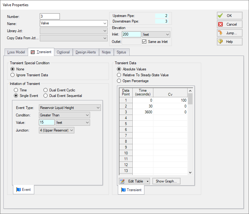
Figure 2: Valve closing Event Transient definitions are made on the Transient tab in the Valve Properties window
Fathom will display a T next to the junction label on the workspace when a transient has been defined for a junction.
ØTurn on Show Object Status from the View menu to verify if all data is entered. If so, the Pipes and Junctions group in Analysis Setup will have a check mark. If not, the uncompleted pipes or junctions will have their number shown in red. If this happens, go back to the uncompleted pipes or junctions and enter the missing data.
Step 8. Run the Model
Click Run Model on the toolbar or from the Analysis menu. This will open the Solution Progress window. This window allows you to watch as the AFT Fathom solver converges on the answer. This model runs very quickly. Now view the results by clicking the Output button at the bottom of the Solution Progress window.
Step 9. Examine the Output
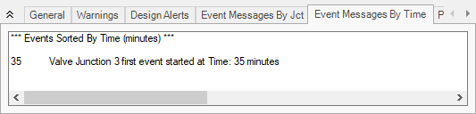
When junction event transients occur, these events are recorded and displayed in the general output section of the Output Window. The events are displayed on two different tabs. The first tab sorts the events by junction number, and the second tab sorts the events by time, in the order in which they occur. The tabs are shown in Figure 3:
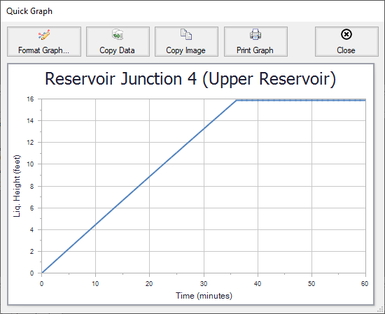
A Quick Graph plot of the liquid height in the reservoir, shown in Figure 4, shows that the final liquid height in the Upper Reservoir is about