Variable Demand - XTS (English Units)
Variable Demand - XTS (Metric Units)
Summary
This example uses a pump transient to initiate auxiliary pump start up for a system with variable demands to ensure adequate pressure drop across a control valve. Additional loads will be added to the system every 30 seconds, until the control valve open percentage exceeds 50%. At that time, the auxiliary pump will start to handle the additional capacity.
Note: This example can only be run if you have a license for the XTS module.
Topics Covered
-
Defining Control Valve Event Transient
-
Understanding Transient Output
-
Using Transient Graphs
Required Knowledge
This example assumes the user has already worked through the Walk-Through Examples section, and has a level of knowledge consistent with the topics covered there. If this is not the case, please review the Walk-Through Examples, beginning with the Beginner: Three Reservoir Model example. You can also watch the AFT Fathom Quick Start Video Tutorial Series on the AFT website, as it covers the majority of the topics discussed in the Three-Reservoir Model example.
In addition, it is assumed that the user has worked through the Beginner: Filling a Tank - XTS example, and is familiar with the basics of XTS transient analysis.
Model File
This example uses the following file, which is installed in the Examples folder as part of the AFT Fathom installation:
-
US - Variable Demand - XTS.fth
Step 1. Start AFT Fathom
From the Start Menu choose the AFT Fathom 12 folder and select AFT Fathom 12.
To ensure that your results are the same as those presented in this documentation, this example should be run using all default AFT Fathom settings, unless you are specifically instructed to do otherwise.
Step 2. Define the Modules Panel
Open Analysis Setup from the toolbar or from the Analysis menu. Navigate to the Modules panel. For this example, check the box next to Activate XTS and select Transient to enable the XTS module for use. A new group will appear in Analysis Setup titled Transient Control. Click OK to save the changes and exit Analysis Setup. Open the Analysis menu to see the new option called Time Simulation. From here you can quickly toggle between Steady Only mode (normal AFT Fathom) and Transient (XTS mode).
Step 3. Define the Fluid Properties Group
-
Open Analysis Setup from the toolbar or from the Analysis menu.
-
Open the Fluid panel then define the fluid:
-
Fluid Library = AFT Standard
-
Fluid = Water (liquid)
-
After selecting, click Add to Model
-
-
Temperature = 70 deg. F
-
Step 4. Define the Pipes and Junctions Group
At this point, the first two groups are completed in Analysis Setup. The next undefined group is the Pipes and Junctions group. To define this group, the model needs to be assembled with all pipes and junctions fully defined. Click OK to save and exit Analysis Setup then assemble the model on the workspace as shown in the figure below.
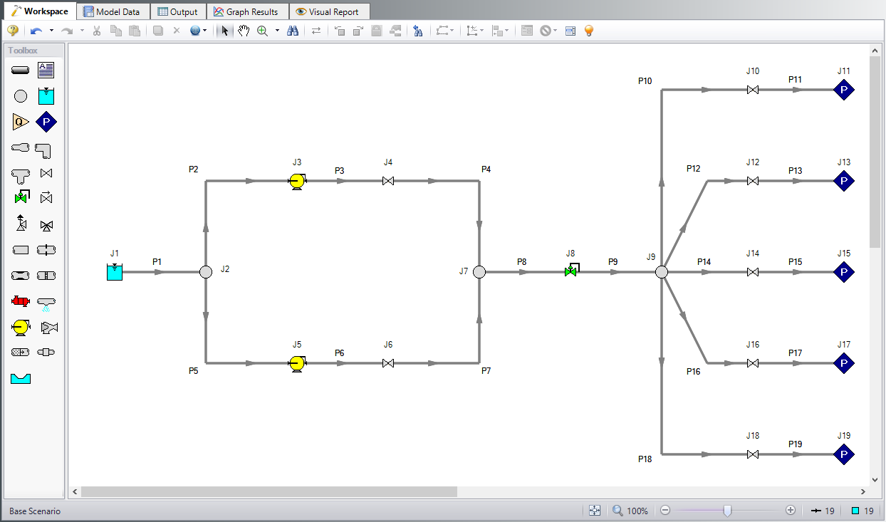
The system is in place but now we need to enter the properties of the objects. Double-click each pipe and junction and enter the following properties. The required information is highlighted in blue.
Pipe Properties
-
Pipe Model tab
-
Pipe Material = PVC - ASTM
-
Pipe Geometry = Cylindrical Pipe
-
Size = 4 inch
-
Type = schedule 40
-
Friction Model Data Set = Standard
-
Lengths =
-
| Pipe | Length (feet) |
|---|---|
| 1-7 & 10-19 | 10 |
| 8 & 9 | 50 |
Junction Properties
-
J1 Reservoir
-
Tank Model = Finite Open Tank
-
Known Parameters Initially = Liquid Surface Level & Surface Pressure
-
Cross-Sectional Area = Constant, 20 feet2
-
Liquid Level Specification = Height from Bottom
-
Liquid Height = 5 feet
-
Liquid Surface Pressure = 0 psig
-
Tank Height = 5 feet
-
Pipe Depth = 5 feet
-
Tank Bottom Elevation = 0 feet
-
-
J2, J7, & J9 Branches
-
Elevation = 0 feet
-
-
J3 & J5 Pumps
-
Inlet Elevation = 0 feet
-
Pump Model = Centrifugal (Rotodynamic)
-
Analysis Type = Pump Curve
-
Pump Curve Data =
-
| Volumetric | Head |
|---|---|
| gal/min | feet |
| 0 | 80 |
| 125 | 90 |
| 250 | 50 |
-
Curve Fit Order = 2
-
J4 & J6 Valves
-
Inlet Elevation = 0 feet
-
Valve Data Source = User Specified
-
Loss Model = Cv
-
Loss Source = Fixed Cv
-
Cv = 100
-
-
J8 Control Valve
-
Inlet Elevation = 0 feet
-
Control Valve Model tab
-
Valve Type = Pressure Reducing (PRV)
-
Always Control (Never Fail) = Unchecked
-
Control Setpoint = Pressure, Static
-
Setpoint = 45 psia
-
Loss When Fully Open = Cv
-
Loss Source = From Open % Table (on Optional Tab)
-
-
Optional tab
-
Open Percentage Data =
-
-
| Open Pct. | Cv |
|---|---|
| 0 | 0 |
| 100 | 100 |
-
J10, J12, J14, J16, & J18 Valves
-
Inlet Elevation = 10 feet
-
Valve Data Source = User Specified
-
Loss Model = Cv
-
Loss Source = Fixed Cv
-
Cv = 10
-
-
J11, J13, J15, J17, & J19 Assigned Pressures
-
Elevation = 10 feet
-
Pressure = 0 psig
-
Pressure Specification = Stagnation
-
Step 5. Define the Transient Control Group
Open Analysis Setup again and navigate to the Simulation Duration panel, part of the Transient Control group.
For this example, with a Start Time of 0 minutes, set the Stop Time to 3 minutes with a time step of 5 seconds. The output will be saved to the output file for every time step.
Step 6. Enter the Transient Data
Valve Transients
Initially, the only flow through the system will be through the J10 Valve. Valves J12, J14, J16, and J18 will start closed, and they will open 30 seconds apart, in sequence. Set the Special Condition for Valves J12, J14, J16, and J18 to Closed on the Valve Properties Optional tab.
The valve opening transient for Valve J12 is shown in Figure 2. Valves J14, J16, and J18 should be set up with the same opening transient, and by adding 30 seconds to the Time Absolute event for each valve so that valve J14 opens at 60 seconds, valve J16 opens at 90 seconds, and valve J18 opens at 120 seconds.
Note that a red XT will now be displayed next to the junction labels to show that these valves are closed, and have transients applied to them.
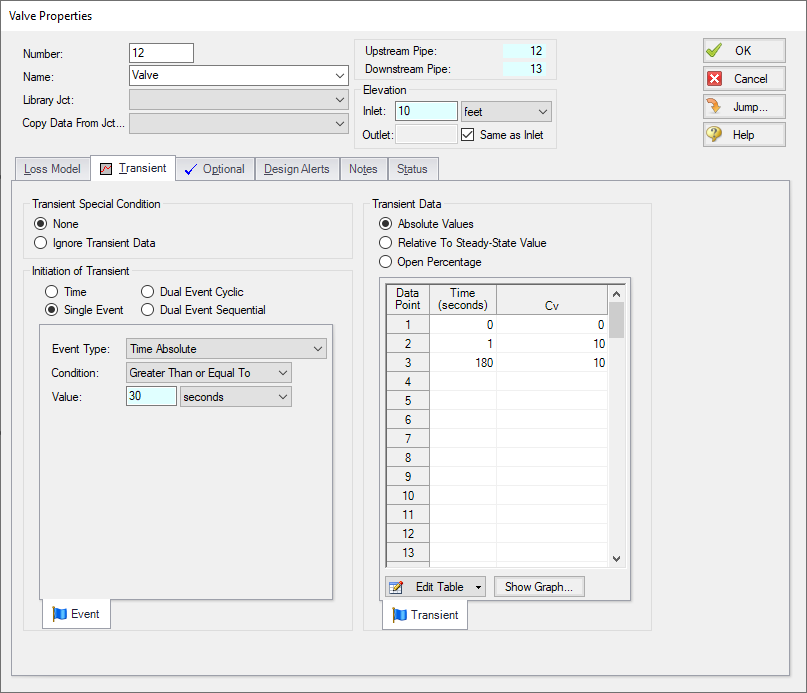
Figure 2: Valve J12-J18 opening transient profiles are defined on the Transient tab on the Valve Properties window
Pump Transient
Pump J5 is not operating at the beginning of this simulation. On the Optional tab of the Pump Properties window set the Pump J5 Special Condition to Pump Off With Flow Through. The pump is set to start when the open percentage of Control Valve J8 exceeds 50%. The transient event definition and pump startup profile are shown in Figure 3.
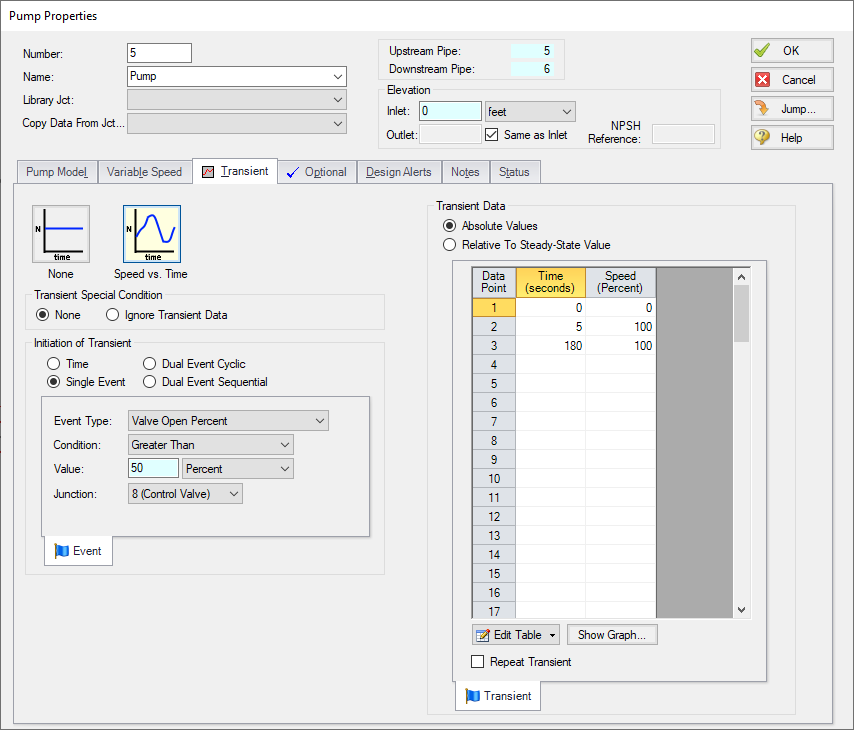
Figure 3: Pump J5 transient startup profile is defined on the Transient tab on the Pump Properties window
Isolation Valve J6 should be closed initially to prevent flow through the leg while Pump J5 is not operating. Do this by setting the Valve J6 Special Condition to Closed on the Optional tab. Valve J6 will open when Pump J5 starts. To do this, use the same transient event as defined for Pump J5. This is shown in Figure 4.
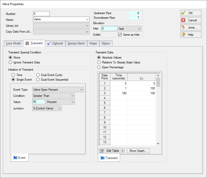
Figure 4: Valve J6 opening transient profile is defined on the Transient tab on the Valve Properties window
ØTurn on Show Object Status from the View menu to verify if all data is entered. If so, the Pipes and Junctions group in Analysis Setup will have a check mark. If not, the uncompleted pipes or junctions will have their number shown in red. If this happens, go back to the uncompleted pipes or junctions and enter the missing data.
Step 7. Run the Model
Click Run Model on the toolbar or from the Analysis menu. This will open the Solution Progress window. This window allows you to watch as the AFT Fathom solver converges on the answer. This model runs very quickly. Now view the results by clicking the Output button at the bottom of the Solution Progress window.
Step 8. Examine the Output
The occurrence of the transient events is recorded on two tabs in the General Output section. The first tab sorts the events by junction, and the second tab sorts the events chronologically. Figure 5 shows the chronological ordering of the transient events for this run. This output shows the downstream valves opening at 30-second intervals. It also shows that Pump J5 started 65 seconds into the run, and the isolation valve J6 also opened at 65 seconds.
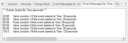
Figure 5: A chronological list of Transient Events is shown in the General Output section of the Output Window
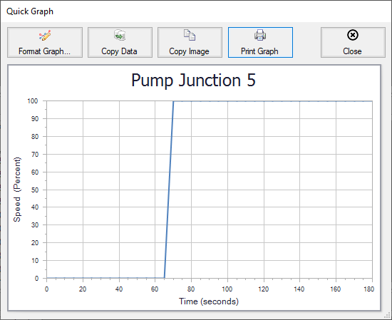
Plotting the speed of Pump J5 vs. time as a Quick Graph from the Output shows the pump starting up at 65 seconds, and coming up to full speed over 5 seconds. This is shown in Figure 6.
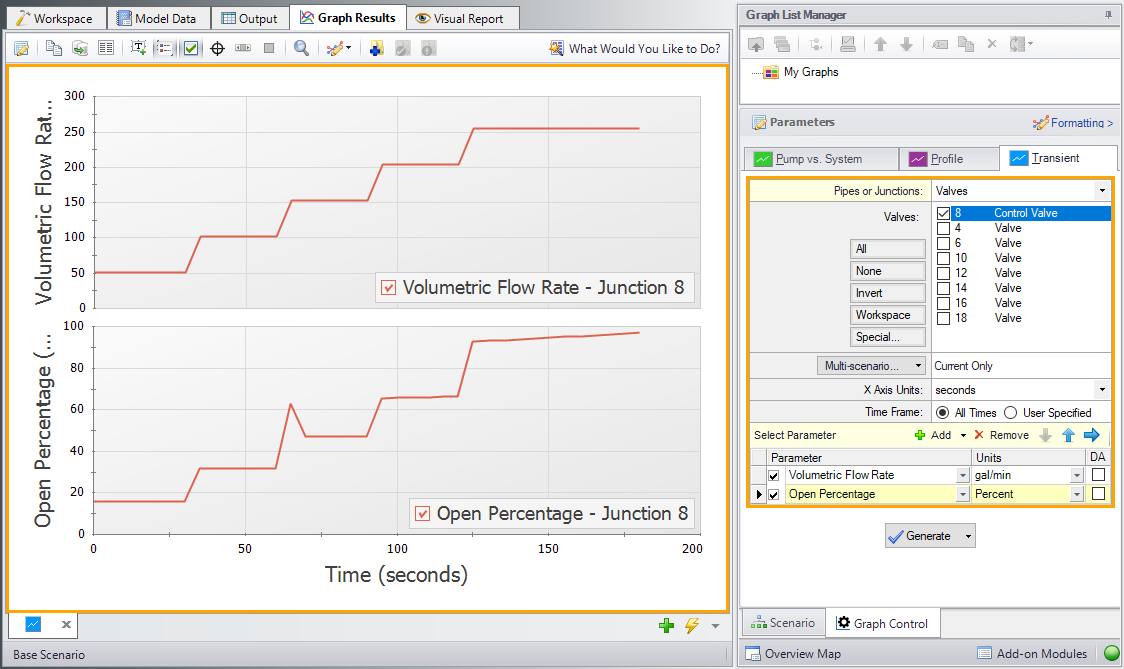
Now go to the Graph Results window. A stacked graph can be made for the Control Valve J8 as shown in Figure 7 to see the affect of the opening valves on the flow rate at the control valve, as well as how the open percent at the control valve responds. It can be seen here that the control valve open percent reaches 50% at 65 seconds, which correlates with the beginning of the pump startup.
To create these stacked graphs, go to the Transient tab in Graph Control. Change the Pipes or Junctions selection to Valves and check the box next the 8, Control Valve. At the bottom, click the Add button next to Select Parameter to add a second parameter to graph. Set the first parameter to Volumetric Flow Rate with