Heat Transfer in Pipes - Detailed Discussion
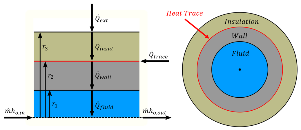
Figure 1: Diagram of a pipe with Heat Tracing and Insulation
There are many possible combinations of heat transfer that can be defined in AFT Fathom. In any of these models there are various heat flows that can be considered.
Figure 1 shows the heat rates for one of the more complex cases – convective heating with a heat trace on the outer face of the pipe wall. Because this is a steady-state problem, any control volume that is drawn around sub-sections or the entire section must have entering heat equal to leaving heat.
Balancing these heat rates and temperatures via iterative methods allows AFT Fathom to come to a unique solution.
Heat Rates
As a hydraulic solver, the primary heat rate of interest is
![]() , the heat added to the fluid itself. Adding heat to the fluid has the effect of raising its temperature.
, the heat added to the fluid itself. Adding heat to the fluid has the effect of raising its temperature.
We can derive an expression for
![]() with the first law of thermodynamics. For convenience, we use specific quantities (per unit mass)
with the first law of thermodynamics. For convenience, we use specific quantities (per unit mass)

The energy e is composed of internal energy u and kinetic energy V2/2. Note that the gravity term gz is neglected from this equation to simplify the derivation.


The work done by the fluid is comprised of pressure work pv and shaft work wshaft

Combining and rearranging

Using the definition of enthalpy


In this analysis, we consider that the velocity through the control volume remains constant. In reality, changing temperature will cause the density of the fluid to change, and thus the velocity. For this reason, pipes in AFT Fathom are thermally sectioned. This means that certain properties are considered constant throughout the section as an approximation – having several sections in a pipe helps increase the accuracy of this approximation.
There is also no shaft work being done on the fluid.

We further assume that this can be treated thermodynamically as a constant pressure process. That is, cp is constant in the thermal section, like density. With this assumption we can use the relationship

To find that

Rather than using specific quantities, it is useful to relate heat rate and mass flow. Multiply both sides by ṁ

The other heat rates in the system can be related to
![]() and other user defined values like
and other user defined values like
![]() or
or
![]() by examining various control volumes and surfaces:
by examining various control volumes and surfaces:

We now have a system of equations that allow us to determine all the heat rates in the system given a mass flow (determined hydraulically), a specific heat (defined versus temperature) and a change in temperature. However, we do not know what this change in temperature is. To find it, we need to relate the surface temperatures to the heat rates.
Surface Temperatures and Resistance
Thermal resistances are useful because they directly relate the heat rate between two points with the temperature between those points.

The value of resistance depends on the mechanism of heat transfer


For conduction, the area and thus resistance changes with increasing r, so an integration must be done


These resistances can all be calculated with user-defined data. AFT Fathom helps simplify this by offering several correlations that can be used to determine the heat transfer coefficients in the above equations from more readily available parameters.
With resistances and
![]() , all the surface temperatures can be determined. By bounding the system with a given Tambient we can work outside in to find the required Tfluid to obtain those heat rates.
, all the surface temperatures can be determined. By bounding the system with a given Tambient we can work outside in to find the required Tfluid to obtain those heat rates.


If the result for Tfluid matches the values used for ΔTfluid used for determining
![]() , the correct solution has been found. If they are different, ΔTfluid needs to be adjusted and the process repeated until reaching a stable solution.
, the correct solution has been found. If they are different, ΔTfluid needs to be adjusted and the process repeated until reaching a stable solution.
Overall Heat Transfer
Wherever there are sequential thermal losses, it is convenient to combine these losses. This is straightforward:

Additionally, an overall heat transfer coefficient U can be defined which behaves similarly to h or k

Using the heat rate and resistance relationship, as well as the fact the heat transfer is into the fluid


Transforming the equation into a differential form on radius and length

Rearranging and integrating


We arrive at an expression relating the temperature change along the pipe and temperature change through the pipe:

Thermal resistances depend on the conduction and convection coefficients k and h which can be directly specified or calculated via a correlation.
The convection coefficient for internal fluid convection can be calculated with the Gnielinski Correlation or the Dittus-Boelter Correlation found in Incropera. These correlations determine the Nusselt number of the fluid – a ratio of convective to conductive heat transfer. Conductive properties are required input – with a Nusselt number and conductivity defined, the convection coefficient can be calculated.

These correlations also make use of the Prandtl number, a ratio of viscous diffusion to thermal diffusion.

Gnielinski

Dittus-Boelter

External convection behavior differs from the above. AFT Fathom provides the Churchill-Bernstein correlation for determining a convection coefficient from ambient temperature and fluid velocity. This correlation can be used for pipes over which boundary layers develop freely, free of constraints imposed by other surfaces. All of the external fluid properties are evaluated at the film temperature.

Buried Pipe Heat Transfer
Buried Pipe heat transfer is modeled by solving directly for the thermal resistance of the soil layer. AFT Fathom uses a model developed by Eckert and DrakeEckert, E.R.G., and Drake, R., Analysis of Heat and Mass Transfer, McGraw-Hill, New York, NY, 1972. to directly calculate the thermal resistance of soil on top of a pipe for use in the overall thermal resistance network:

In this model, z is the distance between the ground surface and the pipe centerline, while r is the outside radius of the pipe.
Related Blogs
Let the Heat Flow: Modeling Heat Transfer in Pipes in AFT Fathom and AFT Arrow


