Stagnation vs. Static Pressure Boundaries
With two exceptions (to be discussed), all pressure-type boundary conditions in AFT Fathom are stagnation. This works very well for things such as storage tanks, cooling ponds, lakes, etc., where the volume associated with a pressure is large and will not change (significantly) with time. These boundaries have no velocity associated with them, and using stagnation pressure is thus appropriate. These boundary conditions are most clearly rendered in AFT Fathom by use of a Reservoir junction.
Consider the reservoir and connected pipe in Figure 1. When the liquid in a reservoir flows into connecting pipes, the static pressure immediately drops due to the increase in velocity.
It is tempting to say that because there is no velocity in the reservoir, then it does not matter whether the reservoir boundary pressure is considered as a static or stagnation pressure because they are equal. This is a misconception. The pressure boundary condition in an AFT Fathom model is applied at the exit of the reservoir, not within the reservoir itself. Inside the reservoir, the static and stagnation pressures are the same, but they are not the same at the exit - they differ by the amount of the dynamic pressure.
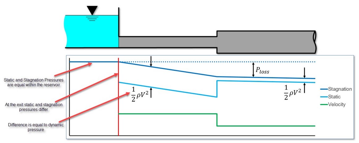
Figure 1: Pressure profile along horizontal pipe shown
The choice of either stagnation or static pressure as a boundary condition depends on whether there is a velocity associated with the pressure that is specified. If the pressure is in a vessel or large (lower velocity) header, then a stagnation pressure is appropriate. If the pressure is in a pipe somewhere in the middle of a system, static pressure is more suited.
Pressure boundary conditions with no velocity are more common across all piping industries, and are usually appropriate. However, this is not always the case.
When to use Static Pressure
Now let's consider the application of a true static pressure boundary condition. A static boundary condition has a unique velocity associated with it. The Bernoulli equation, which in this integrated form applies only to incompressible flow, is given by:

From this equation it can be seen that application of the static pressure is not sufficient to specify location 1. The velocity and elevation is also required.
In AFT Fathom, elevation data is entered for junctions. The pipes adopt the elevation of the junction to which they are connected.
But where does the velocity information for the Bernoulli equation come from? One might respond that it can be obtained from the flow rate. But this raises another question: what if the flow rate isn’t known? Put another way, what if the flow rate is what we are solving for?
When the user supplies a stagnation pressure boundary condition, AFT Fathom can use Equation 6 in the Network Solution Methodology topic. Here, no velocity information is required. A stagnation pressure boundary can thus be supplied to multiple pipes that might have different velocities. That is why the same reservoir junction can connect with multiple pipes.
However, if the user specifies a static pressure as the boundary condition, to apply Equation 4 in the Network Solution Methodology topic, a unique velocity must be supplied. Thus, it is only possible to connect a static pressure to a single pipe with a unique velocity.
Important: A static pressure boundary has a unique velocity associated with it, and can thus connect to only one pipe.
Where would one find a static pressure boundary? The best example is when the boundary condition is inside a pipe. A pipe system model can start and end anywhere it is convenient for the user. It may be convenient to not start the model at the physical boundary (such as a tank) but at a particular location in the pipe system. This could be, for example, at the location of a pressure measurement. Or it could be at the boundary of the pipe system for which your company is responsible, with another company responsible for what is on the other side of that boundary.
If one needs to model such a situation, the Assigned Pressure junction allows one to model either a static or stagnation pressure. The default stagnation pressure allows connection of up to 25 pipes. If static pressure is chosen, only one connecting pipe is allowed.
Static Pressure at Pressure Control Valves
Another example of static pressure is at pressure control valves. For pressure control valves (i.e., PRV’s and PSV’s) the default control pressure is static pressure. The reason is that the measured pressure that provides feedback to the controller will typically be a static pressure measurement. You have the option of modeling pressure control valves as either static or stagnation pressure.


