Gas Turbine Fuel System Example (Metric Units)
For the US units version of this example, click here.
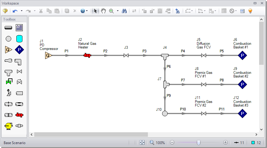
The combustion baskets in a natural gas fuel system are fed by a positive displacement compressor. The natural gas is preheated by a heat exchanger before passing through the three control valves, with each feeding a separate combustion basket. One of the control valves experiences a nearly instantaneous closure. The objective is to determine the maximum fluid temperature reached during the transient, both in the entire system, and at the inlets of the combustion baskets. The effect of this transient event on the temperature, pressure, and velocity of the system should be observed.
As the design engineer, you are also responsible for evaluating the sensitivity of the results to the Minimum Number of Sections Per Pipe parameter.
Topics Covered
-
Modeling a valve closure as a transient event
-
Modeling a heat exchanger
-
Using the Scenario Manager
-
Importance of the Estimated Maximum Temperature During Transient setting
-
Finding the max and min values for transient parameters
-
Creating animated profile graphs
Required Knowledge
This example assumes that the user has some familiarity with AFT xStream such as placing junctions, connecting pipes, and entering pipe and junction properties. Refer to the
Model File
A completed version of the model file can be referenced from the Examples folder as part of the AFT xStream installation:
C:\AFT Products\AFT xStream 3\Examples
Step 1. Build the model
A. Place the pipes and junctions
-
ØIn the Workspace window, assemble the model as shown in Figure 1.
B. Enter the pipe and junction data
The system is in place but now the input data for the pipes and junctions needs to be entered. Enter the following data in each Pipe and Junction Properties window.
All Pipes are Stainless Steel - ANSI, Schedule 10S, and have standard roughness. The rest of the pipe information is as follows:
| Pipe # | Size (inches) | Length (meters) |
|---|---|---|
| 1 | 8 | 23 |
| 2 | 8 | 7.5 |
| 3 | 8 | 1.5 |
| 4 | 5 | 1.5 |
| 5 | 5 | 1.5 |
| 6 | 8 | 1.5 |
| 7 | 5 | 1.5 |
| 8 | 5 | 1.5 |
| 9 | 8 | 1.5 |
| 10 | 5 | 1.5 |
| 11 | 5 | 1.5 |
Because several of the pipes are the same, you can use the Global Pipe Edit tool to speed up the process of entering the data. The Global Pipe Edit tool allows you to apply changes to multiple pipes at the same time.
-
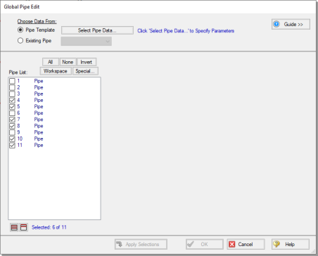
ØSelect Global Pipe Edit either from the Edit menu, or by selecting the Global Edit dropdown on the toolbar (blue globe symbol) and selecting the Global Pipe Edit option. This will open the Global Pipe Edit window.
-
ØSelect Pipes P4, P5, P7, P8, P10, and P11 from the list of pipes as shown in Figure 2.
-
ØClick the Select Pipe Data button. This will open a template Pipe Properties window for entering the data to be applied to all of the selected pipes.
-
ØFill out the data for the selected pipes. When you have entered all of the data for the pipes, close the Pipe Properties window by selecting OK. The Global Pipe Edit window will now display a list of all of the parameters that may be applied to the selected pipes. The parameters are categorized as they are displayed on the tabs in the Pipe Properties window.
-
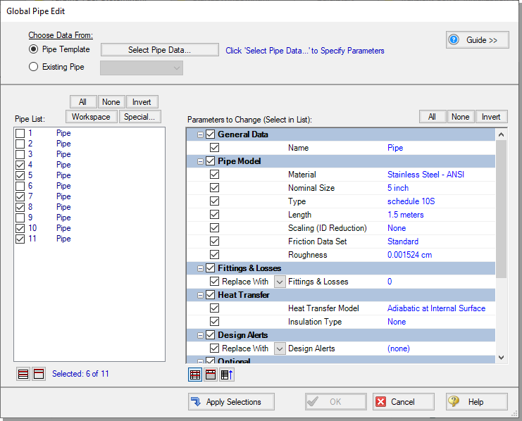
ØSelect the All button above the Parameters to Change list, since for this example, you want all of the parameters for all of the selected pipes to be updated to the specified values. The Global Pipe Edit window should now appear as shown in Figure 3.
-
ØApply the changes to the selected pipes by clicking the Apply Selections button. AFT xStream will notify you that the changes have been completed with a message in the bottom-left of the Global Pipe Edit window. At this point, all of the changes have been applied but not saved. If you wish to cancel all of the changes you just implemented, you may do so by clicking Cancel on the Global Pipe Edit window.
-
ØSave the applied changes by clicking OK.
Note: The Guide button in the Global Edit windows may be used as a reminder of the required steps for the global edit process if needed.
-
Assigned Flow J1
-
Name = PD Compressor
-
Elevation =
-
Mass Flow Rate =
Note: Be advised that the unit for mass flow is not the default, it is
-
Temperature =
-
-
Heat Exchanger J2
-
Name = Natural Gas Heater
-
Elevation =
-
K = 6.6
-
Steady Heat Rate =
-
-
Valve J3
-
Elevation =
-
Kv = 8650
-
xT = 0.3
-
-
Valve J5
-
Name = Diffusion Gas FCV
-
Elevation =
-
Kv = 80
-
xT = 0.7
-
-
Valve J8
-
Name = Premix Gas FCV #1
-
Elevation =
-
Kv = 170
-
xT = 0.7
-
-
Valve J11
- Name = Premix Gas FCV #2
-
Elevation =
-
Kv = 170
-
xT = 0.7
-
Click on the Transient Tab and enter the following data:
| Time (seconds) | Kv | xT |
|---|---|---|
| 0 | 170 | 0.7 |
| 0.01 | 0 | 0.7 |
| 2 | 0 | 0.7 |
-
Assigned Pressures J6, J9, J12
-
J6 Name = Combustion Basket #1
-
J9 Name = Combustion Basket #2
-
J12 Name = Combustion Basket #3
-
Elevation =
-
Stagnation Pressure =
-
Temperature =
-
-
Junctions J4, J7, J10
-
Elevation =
-
C. Check if the pipe and junction data is complete
-
ØOpen the List Undefined Objects window from the View menu or the Workspace Toolbar to verify if all pipes and junctions are specified. If not, the incomplete pipes or junctions will be listed. If undefined objects are present, go back to the incomplete pipes or junctions and enter the missing data.
Step 2. Specify Analysis Setup
-
ØOpen the Analysis Setup window by clicking Analysis Setup on the Common Toolbar.
-
ØSelect Methane from the AFT Standard fluid library, and click the Add to Model button.
Note: Methane is used to approximate natural gas in order to minimize the run time. This is typically a fair assumption for preliminary runs. If you need to model a real natural gas mixture, such as for a final run, then the NIST REFPROP library or the optional Chempak add-on can be used. Be aware that mixtures with multiple components may drastically increase the runtime. Limiting the mixture to 3 or 4 components is advised.
B. Specify the Pipe Sectioning and Output panel
Note: If following along in the completed model file, the Estimated Maximum Pipe Temperature During Transient will have a different value. This will be discussed in later steps.
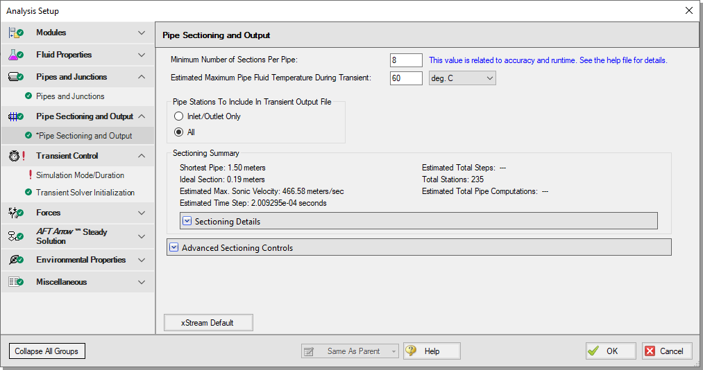
Figure 4: Sectioning panel
C. Specify the Simulation Mode/Duration panel
-
ØEnter a Stop Time of 2 seconds on the Simulation Mode/Duration panel from the Transient Control group. Verify the Time Simulation is set to Transient. Click the OK button.
Step 3. Create scenarios to model different sectioning setups
A. Create scenarios
In this model, the following three types of Sectioning cases for the system are to be evaluated:
-
8 Sections Minimum per Pipe
-
4 Sections Minimum per Pipe
-
2 Sections Minimum per Pipe
To evaluate the three cases, we will utilize the Scenario Manager to create three scenarios for the three cases.
Open the Scenario Manager on the Quick Access Panel. Create a child scenario by either right-clicking on the Base Scenario and then selecting Create Child, or by first selecting the Base Scenario on the Scenario Manager on the Quick Access Panel and then selecting the Create Child icon  . Enter the name 8 Sections Minimum Per Pipe in the Create Child Scenario window, and select the OK button. The new 8 Sections Minimum Per Pipe scenario should now appear in the Scenario Manager on the Quick Access Panel below the Base Scenario. Select the Base Scenario and create another child named 4 Sections Minimum Per Pipe. Finally, create one more child and call it 2 Sections Minimum Per Pipe. The Child Scenarios should now be displayed as shown in Figure 5.
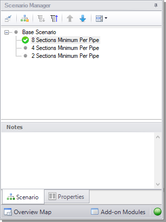
Figure 5: Create model variants and keep them organized using the Scenario Manager on the Quick Access Panel
B. Set up scenarios
Child scenarios inherit data from their ancestor scenarios. As long as the data has not been modified in a child scenario, data parameters in the child scenario will have the same value as their parent. Scenarios can be loaded onto the Workspace by double-clicking their name in the Scenario Manager. The currently loaded scenario is indicated in the scenario tree with a green circle with a checkmark (Figure 5). Since the Base Scenario already has been set up with 8 Minimum Sections Per Pipe, the 8 Sections Minimum Per Pipe child does not need to be modified.
-
ØLoad the 4 Sections Minimum Per Pipe scenario by double-clicking the name in the Scenario Manager. Open the Analysis Setup window from the Common Toolbar. Open the Pipe Sectioning and Output panel and then click OK.
-
ØChange the Minimum Number of Sections Per Pipe to 4 from the Pipe Sectioning and Output panel in Analysis Setup, then click OK. The required input for this scenario is now complete.
-
ØRepeat the steps above for the 2 Sections Minimum Per Pipe scenario, and change the value to 2.
Step 4. Run the first scenario
-
ØDouble-click the 8 Sections Minimum Per Pipe scenario in the Scenario Manager.
-
ØClick the Run Model button on the Common Toolbar or select the option from the Analysis menu. AFT xStream will prompt you to save the model if you have not done so already, then will open the Solution Progress window.
Step 5. Review the results
-
ØClick the Output button. This will take you to the Output window, which will display any warnings if they exist. There should be a warning indicating that the maximum transient pipe temperature was higher than the estimate as well as a caution that the maximum transient pipe mach number was significantly lower than the estimate (see Figure 6). The Estimated Maximum Pipe Temperature During Transient is critical to the calculation of transient conditions due to its necessity in the Method of Characteristics.
The Estimated Maximum Pipe Temperature During Transient is used to calculate the sonic velocity of the fluid, which is then used to create the upper boundary of the characteristic grid. If the maximum temperature during the transient exceeds the specified Estimated Maximum Pipe Temperature During Transient and the flow is sonic, the Method of Characteristics may have to extrapolate data, which can lead to instability and will stop the transient solver. In this model, sonic velocity was not reached when the temperature was higher than the estimated maximum. However, to ensure that this model can handle sonic flow, we will re-run the model with a higher Estimated Maximum Pipe Temperature During Transient.
The Maximum Transient Pipe Mach Number warning indicates that error could be introduced through having a Mach Number substantially lower than the Maximum Transient Pipe Mach Number used for the calculation (in this case, the xStream default value of one). This caution will be ignored in this example for simplicity.
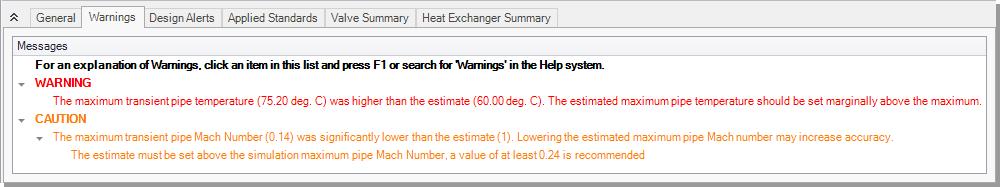
Figure 6: The maximum transient pipe temperature exceeds estimated maximum temperature warning indicates that the model is at risk of instability if changes are made
Step 6. Adjust the Pipe Sectioning panel
-
ØDouble-click the Base Scenario in the Scenario Manager. Open the Analysis Setup window from the Common Toolbar and select Change the Click OK.
-
ØChange the Estimated Maximum Pipe Temperature During Transient to
Important: Making this change in the Base Scenario will save time since it will propagate the change to all scenarios automatically.
Step 7. Re-run the model and review results
A. Review Output window
-
ØRe-run the 8 Sections Minimum Per Pipe scenario, then proceed to the Output window. There should be a caution indicating that the maximum transient pipe mach number was significantly lower than the estimate. Disregard this caution as discussed previously.
ØSelect the Transient Max/Min tab as shown in Figure 7. Here we can see the maximum static temperatures in the pipes (scroll to the right in the Pipes section of the Output). Note that the values here are accounting for the entire length of the pipe, and the corresponding Station at which the max/min values occurred is reported.
The max static temperature for the entire system occurs at the inlet of Pipe P2 (Station 0), with a value of about
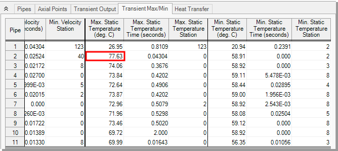
Figure 7: Transient Max/Min tab in the Output window
B. Graph the results
Go to the Graph Results window by clicking on the Graph Results tab or pressing CTRL+G on the keyboard.
-
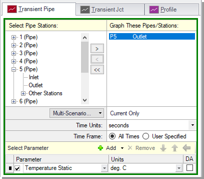
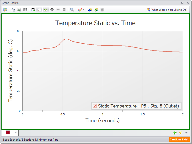
ØCreate a graph that shows the temperature over time at the entrance to Combustion Basket #1 using the following steps (Figure 8):
-
From the Graph Control tab on the Quick Access Panel, select the Transient Pipe tab
-
Select Pipe P5 and add the outlet station
-
Verify that the time units are set to seconds
-
In the Parameters definition area, select Temperature Static with units of deg.
-
Click the Generate button
-
ØRight-click on the resulting graph and select Show Cross Hair, or enable it via the icon on the Graph Toolbar. Moving your mouse cursor over the graph will display the numerical values of the graph data points. This can be used to find the max value, or you can right-click on the graph and select Copy X-Y Data, which can be pasted into Excel or other software utilities for further inspection.
The max temperature at the inlet of Combustion Basket #1 is about
Note: The Assigned Pressure junctions in this model were defined with Stagnation Temperature. Therefore, the Static Temperature will be lower than the Stagnation value, as is seen in Figure 9. In the case of Pipe P11 where the flow is zero after the valve closure, the Static and Stagnation Temperatures will be equal.
To easily recreate this graph in the other scenarios or in the future, it can be added into the Graph List Manager on the Quick Access Panel.
-
ØRight-click the graph and select Add Graph to List from the context menu, or use the icon from the Graph Results Toolbar
 . Give the graph a name, such as “Combustion Basket #1 Temperature vs Time”, then click OK. The graph will be added to the currently selected folder in the Graph List Manager. Note that graphs added to the Graph List Manager are not permanently saved until the model is saved again. Also be aware that only the graph settings are saved as opposed to the graph data.
 -
ØCreate the same graph above for Combustion Basket #2 and #3, and save them as Graph List Items. Combustion Basket #2 corresponds to the Pipe P8 Outlet station, and Combustion Basket #3 corresponds to the Pipe P11 Outlet station. Combustion Basket #2 will have a similar graph with a slightly lower maximum. Combustion Basket #3 will have a flat graph due to the valve closure, and the temperature settles out to the boundary condition of the J12 Assigned Pressure since Pipe P11 is adiabatic with no heat transfer.
AFT xStream can animate output along pipeline paths in your model in the Graph Results window. This feature can help you understand how your system will respond when a transient event occurs. You can also animate multiple graphs at the same time.
Here, you will animate the temperature static, pressure static, and velocity along the flow path between the positive displacement compressor and Combustion Basket #1 in order to gain an understanding of how these parameters respond as the control valve closes.
-
ØSpecify the following graph settings (Figure 10):
-
Create a new graph tab by clicking the New Tab button located in the bottom-right (green “+” icon).
-
Select the Profile tab under the Graph Control tab in the Quick Access Panel.
-
Select Pipes P1 through P5.
-
Ensure the Length Units are
-
Select the option to Animate Using Output. To use this feature, data from all pipe stations must be saved (which is the default on the Pipe Sectioning and Output panel), otherwise the option will be grayed out.
-
Ensure that the Animation Time Units are set to seconds.
-
Add two additional parameters using the Add button, and specify the three parameters:
-
Temperature Static with units of deg.
-
Pressure Static with units of
-
Velocity with units of
-
-
Check the Mx and Mn boxes next to the graph parameters to plot the maximum and minimum values on the graph.
-
Click the Generate button.

Figure 10: Graph parameters for Combustion Basket #1 animated profile
Note: Figure 11 have been modified to increase clarity.
Additional animation control features appear at the top of the Graph Results window (Figure 11). Press the Play button and watch the temperature, pressure, and velocity responses move between the maximum and minimum values. This animation can also be recorded to a file.
-
ØAdd the graph to the Graph list manager by either right clicking on the graph or using the Add Graph to List icon. Give it a name, such as "Combustion Basket #1 Animated Profile".
Playing the animation reveals that the highest temperature in the system is observed at the J2 heat exchanger. It should also be noted that the rise to this maximum temperature occurs when the pressure wave from the valve closing passes through this junction. However, this heightened temperature is not immediately seen by the combustion baskets downstream because the gas velocity throughout the system drops immediately following the valve closure. Instead, the heightened temperature moves slowly downstream until the gas wave is reflected at the positive displacement compressor and passes through the heat exchanger going the opposite direction. This causes the local gas velocity to rise and causes the temperature wave to move downstream towards the combustion baskets more quickly. This wave eventually reaches Combustion Basket #1 at around Time = 0.55 seconds, at which point the inlet to the combustion basket reaches its maximum temperature.
Step 8. Run the other scenarios and graph the results
-
ØLoad and run the other two scenarios using the Scenario Manager.
-
ØObserve the Transient Max/Min tab for each scenario, and note the overall system max static temperature. The max temperature and pressure during both the steady-state and the transient simulation can also be found at the bottom of the General tab in the Output. A summary of the system max temperature for each scenario is shown below in Table 2.
-
ØCreate the same graphs from the previous steps for each of the scenarios by double-clicking on the saved Graph List Items in the Graph List Manager.
Table 3: Combustion Basket max static temperatures for the three sectioning counts
Scenario Combustion Basket #1 Max Transient Temperature (deg. Combustion Basket #2 Max Transient Temperature (deg. Combustion Basket #3 Max Transient Temperature (deg. 8 Sections 4 Sections 2 Sections
Conclusion
Use of transient conditions within a valve junction allowed us to model the effects of an unexpected valve closure in a system. The Scenario Manager was used to easily create variations of the model that analyzed the effect of different pipe sectioning. While this example was focused on temperature, it also showed that values such as pressure and velocity can be tracked by AFT xStream. The overall maximum temperature for the system was found in the Transient Max/Min tab of the Output, and also at the bottom of the General tab for each scenario (Table 2). Different pipe sectioning resulted in different max temperatures (Table 3).
Additionally, this example identified the Estimated Maximum Temperature During Transient as a critical variable in the tabulation of the transient results. This value sets the boundary for the characteristic grid used by the Method of Characteristics. If sonic choking occurs at a temperature higher than the estimated maximum, the model may not converge. As such, this value should be conservatively high on early runs of a model and then refined once the temperature that the transient approaches is known.


