Variable Drive - ANS (English Units)
Variable Drive - ANS (Metric Units)
Summary
As seen in other examples, the ANS module can be used to size a system for life cycle cost. The ANS module will size the complete system, pumps and pipes to minimize the total cost of operating the system for the life of the system. Often sizing the pumps and pipes is not enough because the control system is often a large portion of the initial cost and the method of control, flow control valves (FCV) or variable frequency drives (VFD), can have a large impact on the system energy usage. This example will demonstrate how to size pumps and control valves in parallel and then will investigate the savings of using a VFD to control flow instead of a FCV.
Note: This example can only be run if you have a license for the ANS module.
Topics Covered
-
Using Scenarios to size a system for two different sets of system requirements
-
Using Common Size Groups and observing their effect on how well the ANS module can size a system
Required Knowledge
This example assumes the user has already worked through the Walk-Through Examples section, and has a level of knowledge consistent with the topics covered there. If this is not the case, please review the Walk-Through Examples, beginning with the Beginner: Three Reservoir Model example. You can also watch the AFT Fathom Quick Start Video Tutorial Series on the AFT website, as it covers the majority of the topics discussed in the Three-Reservoir Model example.
In addition, it is assumed that the user has worked through the Beginner: Three-Reservoir Problem - ANS example, and is familiar with the basics of ANS analysis.
Since this example employs many concepts from the Cooling System - ANS example, it is recommended to complete that example first before beginning this example.
Model Files
This example uses the following files, which are installed in the Examples folder as part of the AFT Fathom installation:
-
Variable Drive.dat - engineering library
-
Variable Drive - Pump Costs.cst - cost library for Variable Drive.dat
-
Variable Drive - VFD Costs.cst - cost library for Variable Drive.dat
-
Variable Drive - Pipe Costs.cst - cost library for Steel - ANSI pipes
Step 1. Start AFT Fathom
From the Start Menu choose the AFT Fathom 12 folder and select AFT Fathom 12.
To ensure that your results are the same as those presented in this documentation, this example should be run using all default AFT Fathom settings, unless you are specifically instructed to do otherwise.
Step 2. Set up Library Manager
This example uses engineering and cost libraries. It is important that these libraries are added and connected to Fathom for defining the pipes and junction.
Go to the Library menu and open Library Manager. Click Add Existing Library and navigate to the AFT Fathom 12 Examples folder. Select the library Variable Drive.dat and click Open. Make sure that the Variable Drive engineering library in Library Manager has a check mark next to it. The cost libraries will be added later during the Sizing steps.
Step 3. Define the Modules Panel
Open Analysis Setup from the toolbar or from the Analysis menu. Navigate to the Modules panel. For this example, check the box next to Activate ANS and select Network to enable the ANS module for use. A new group will appear in Analysis Setup titled Automatic Sizing. Click OK to save the changes and exit Analysis Setup. A new Primary Window tab will appear between Workspace and Model Data titled Sizing. Open the Analysis menu to see the new option called Automatic Sizing. From here you can quickly toggle between Not Used mode (normal AFT Fathom) and Network (ANS mode).
Step 4. Define the Fluid Properties Group
-
Open Analysis Setup from the toolbar or from the Analysis menu.
-
Open the Fluid panel then define the fluid:
-
Fluid Library = User Specified Fluid
-
Name = Lube Oil
-
Density = 0.7 S.G. water
-
Dynamic Viscosity = 0.29 kg/sec-m
-
Step 5. Define the Pipes and Junctions Group
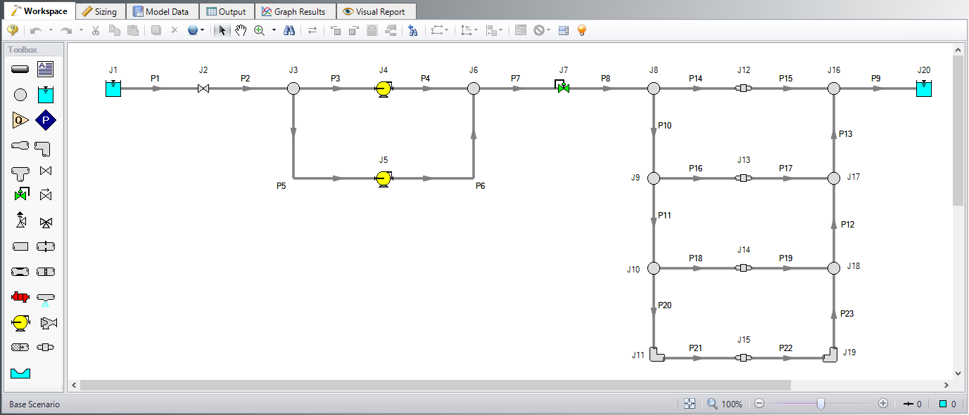
At this point, the first two groups are completed in Analysis Setup. The next undefined group is the Pipes and Junctions group. To define this group, the model needs to be assembled with all pipes and junctions fully defined. Click OK to save and exit Analysis Setup then assemble the model on the workspace as shown in the figure below.
Pipe Properties
-
Pipe Model tab
-
Pipe Material = Steel - ANSI
-
Pipe Geometry = Cylindrical Pipe
-
Size = 4 inch
-
Type = schedule 40
-
Friction Model Data Set = Standard
-
Lengths =
-
| Pipe | Length (feet) |
|---|---|
| 7 | 4 |
| 3-4 | 6 |
| 2, 5-6, 10-13, 20, 23 | 10 |
| 8 | 15 |
| 1, 14-19, 21-22 | 20 |
| 9 | 50 |
Junction Properties
-
J1 Reservoir
-
Name = Lube Oil Supply Tank
-
Liquid Surface Elevation = 20 feet
-
Liquid Surface Pressure = 1 atm
-
Pipe Depth = 10 feet
-
-
J2 Valve
-
Name = Isolation Valve
-
Inlet Elevation = 0 feet
-
Valve Data Source = User Specified
-
Loss Model = K Factor
-
K = 0.15
-
-
All Branches
-
Elevation = 0 feet
-
-
J4 & J5 Pumps
-
J4 Name = Primary Pump
-
J5 Name = Auxiliary Pump
-
Library Jct = Pump 2000 gal/min Sizing
-
Inlet Elevation = 0 feet
-
J5 Special Condition = Pump Off No Flow
-
-
J7 Control Valve
-
Name = 2000 gal/min Control
-
Inlet Elevation = 0 feet
-
Valve Type = Constant Pressure Drop (PDCV)
-
Control Setpoint = Pressure Loss
-
Pressure Drop = 10 psid
-
-
J11 & J19 Bend
-
Inlet Elevation = 0 feet
-
Type = Standard Elbow (knee, threaded)
-
Angle = 90 Degrees
-
-
J12-J15 General Components
-
J12 Name = Generator #1
-
J13 Name = Generator #2
-
J14 Name = Generator #3
-
J15 Name = Generator #4
-
Library Jct = US - Generator
-
Inlet Elevation = 0 feet
-
-
J20 Reservoir
-
Name = Return Tank
-
Liquid Surface Elevation = 15 feet
-
Liquid Surface Pressure = 1 atm
-
Pipe Depth = 15 feet
-
The system supplies lube oil to a bank of four generators. Each generator requires a flow rate of
The system uses the following specifications:
-
Minimum 10 psid drop across the flow control valve
-
Flow rate at each generator must be between 450 and 550 gal/min
-
The cost of the auxiliary pump and piping must be included in the sizing.
-
The pump is expected to be about 80% efficient.
-
The system uses lube oil with a specific gravity of 0.7 and viscosity of 0.29 kg/s-m.
Step 6. Configure Sizing Settings
We want to first size our system to determine the required pump parameters, which will then be used to choose a pump model and perform a final sizing calculation.
To start, set up the model to size the pump system for life cycle cost. Select the Sizing tab.
A. Sizing Objective
The Sizing Objective panel should be selected by default from the navigation panel. Choose the settings as follows:
For the Sizing Option choose Perform Sizing.
For the Objective, choose Monetary Cost, and select the Minimize option from the drop-down list.
Under Options to Minimize Monetary Cost, choose Size for Initial and Recurring Costs. This should automatically configure the Cost Objective table to include the material, installation, and energy costs in the sizing.
Define a 10 year System Life.
For the Energy Cost area choose Use This Energy Cost Information, with a cost of 0.06 U.S. Dollars Per kW-hr.
B. Size/Cost Assignments
On the Sizing Navigation panel go to the Size/Cost Assignments panel.
We are designing a new system, so we want to include all of the pipes in the model for sizing.
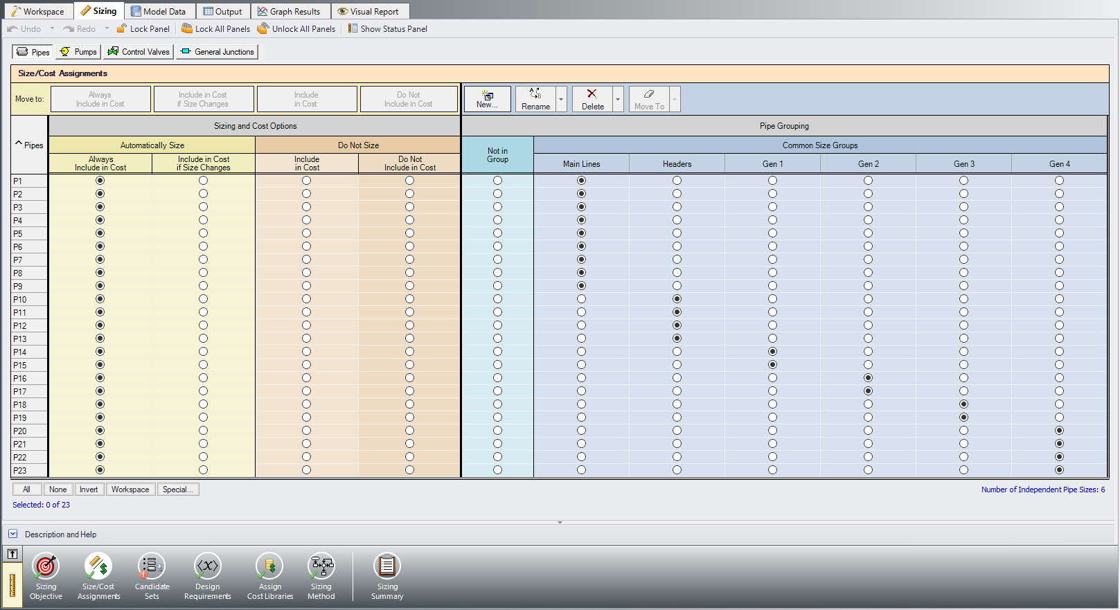
ØSelect the All button at the bottom of the panel to select all pipes, then click Always Include in Cost at the top of the table to move all pipes to be included in the sizing calculation.
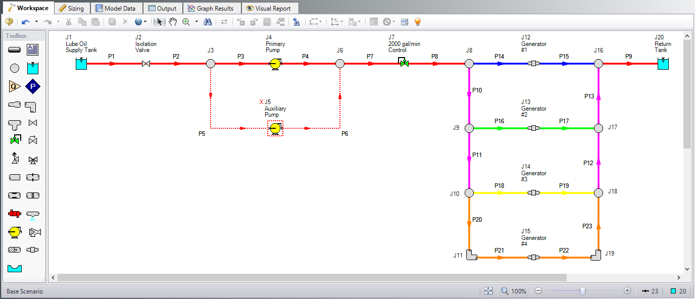
To decrease the analysis speed and reduce complexity, it is useful to create Common Size Groups to group the pipes in different sections of the model. For this system we want to create six groups to be sized, as can be seen in Figure 2 based on the pipe coloring, and Figure 3 based on the table. The groups were chosen by considering sections of pipe which would logically have similar demands due to the flow capacity and connected junctions.
Create each of the groups by selecting the appropriate pipes in the Workspace, then right-clicking on the Workspace and choosing Add Pipes to Common Size Group -> New Group and giving the group a name. Alternatively the groups can be created on the Sizing window by clicking New to create and name the group, then adding pipes to the group using the radio buttons. The Size/Cost Assignments panel should appear as shown in Figure 3.
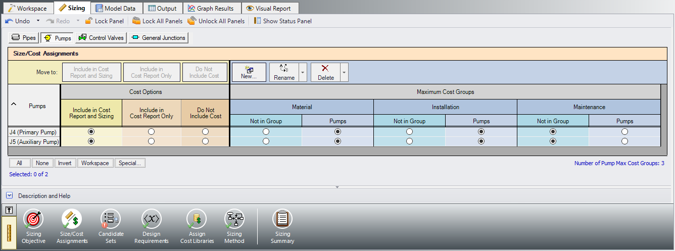
ØClick the Pumps button at the top of the panel to switch to the Pump Size and Cost Assignments. As stated earlier, we want to size both pumps, even though the Auxiliary Pump is not in use, so select Include in Cost Report and Sizing for each of the Pump junctions. Since the pumps are in parallel in this model, it is desired for the pumps to be the same size. This means that they will have the same material and installation costs, though the maintenance cost will be different since the Auxiliary Pump is not regularly used, unlike the Primary Pump. To account for this we will need to create a Maximum Cost Group, which will set both pumps to use the cost information for the most expensive pump in the group. If a Maximum Cost Group is not used, then the Auxiliary Pump will have its material and installation costs set to the lowest possible cost. (The cost at the pump is estimated using power, and the power at the Auxiliary Pump is set at zero since it is not in use during normal operation.)
ØCreate a New Maximum Cost Group named Pumps, and add the Material and Installation costs to it for each of the pumps, but under Maintenance, make sure to leave both pumps in the Not in Group column. The Pumps Size/Cost Assignments should appear as shown in Figure 4.
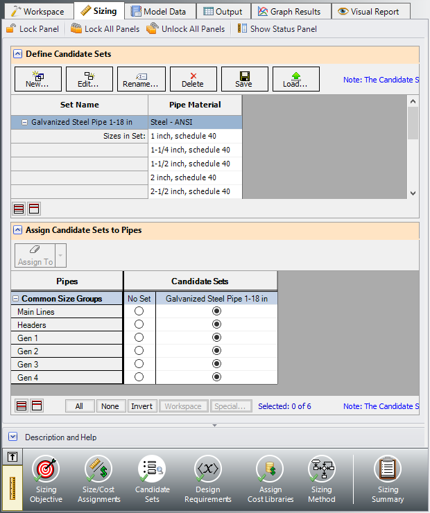
C. Candidate Sets
Go to the Candidate Sets panel.
For this system we will consider a range of Steel-ANSI schedule 40 pipes as candidates. To define this in Fathom, create a new Candidate set as follows:
-
Create a new set by clicking New, and name the set Galvanized Steel Pipe 1-18 in.
-
Select Steel - ANSI as the material from the drop-down list
-
In the Available Material Sizes and Types, expand the sizes for schedule 40, then add each of the sizes from 1 inch to 18 inch by double clicking the names or selecting them and clicking Add>>.
-
Click OK to finish editing the set.
In the bottom section of the panel, assign each of the Common Size Groups to the Galvanized Steel Pipe 1-18 in Candidate Set. The panel should appear as shown in Figure 5.
D. Design Requirements
Go to the Design Requirements panel.
As can be seen above, this model has three given Design Requirements which need to be applied for the generators and control valve. Since we are not able to directly apply a flow rate design requirement on the generators, we will instead apply the flow rate requirements for the generators to the pipes adjacent to the generators. To do this:
-
Make sure the Pipes button at the top of the window is selected.
-
Click New under Define Pipe Design Requirements.
-
Enter the name Max Generator Flow.
-
In the table for Parameter, select Volumetric Flow Rate.
-
For Max/Min, choose Maximum, and enter 550 gal/min.
-
Repeat the process from steps 1-5 to define a Design Requirement for a Minimum generator flow rate of 450 gal/min.
Now that the generator flow rate requirements are defined, apply them to the common size groups for the generator piping (Gen 1, Gen 2, Gen 3 and Gen 4) by checking the appropriate boxes in the Assign Design Requirements to Pipes section.
Click on the Control Valves button and create a New requirement named Min Pressure Drop to set the Pressure Drop Stagnation parameter to a Minimum of
E. Assign Cost Libraries
Go to the Assign Cost Libraries panel. For this model, the engineering and cost libraries have already been created, but we will need to check that they have been connected and applied properly.
ØOpen the Library Manager, and check that the engineering library Variable Drive is connected, indicated by a check mark next to its name. If it is not connected, then check the box next to its name.
Next, connect to the three cost libraries. Click Add Existing Cost Library and navigate to the AFT Fathom 12 Examples folder and add the cost libraries Variable Drive - Pump Costs.cst, Variable Drive - VFD Costs.cst, and Variable Drive - Pipe Costs.cst. The two cost libraries, Variable Drive - Pump Costs and Variable Drive - VFD Costs should be shown indented below the engineering library Variable Drive, and the Variable Drive - Pipe Costs library should be indented below Steel - ANSI. Once all of the necessary libraries have been connected, click OK.
In the Assign Cost Libraries panel for the Pipes, All should be selected for the Galvanized Steel Pipe 1-18 in Candidate Set, with the Variable Drive - Pipe Costs library being applied.
ØClick on the Pumps button to view the cost library assignments for the Pumps. We will only be using Variable Drive - Pump Costs for this scenario, so check the box for this cost library for both J4 and J5 to make sure that we are not applying any extra costs.
F. Sizing Method
Select the Sizing Method button to go to the corresponding panel.
ØChoose Discrete Sizing, since it is desired to select discrete sizes for each of the pipes in the model.
This model contains six design variables and 18 design requirements, so the best methods to choose from will be the MMFD or SQP method.
ØSelect the default method, Modified Method of Feasible Directions (MMFD).
Step 7. Create Scenarios
Before running the model, create two child scenarios, one named Calculate Costs, Do Not Size and the other named FCV Initial Cost Sizing. This will provide a comparison of the initial cost of the model without sizing, to the cost of the sized system.
Load the Calculate Costs, Do Not Size scenario and go to the Sizing window, then to the Sizing Objective panel. Select Calculate Costs, Do Not Size. We will run this scenario first.
Step 8. Run the Model
Click Run Model on the toolbar or from the Analysis menu. This will open the Solution Progress window. This window allows you to watch as the AFT Fathom solver converges on the answer. This model runs very quickly. Now view the results by clicking the Output button at the bottom of the Solution Progress window.
Step 9. Review the Not Sized and Initial Cost Sizing results
You will immediately notice that both minimum and maximum flow design requirements to several generators were violated. However, the flow rates are not too far outside the acceptable range. Either way, the current design is infeasible. Go to the Cost Report tab and note that the total cost is
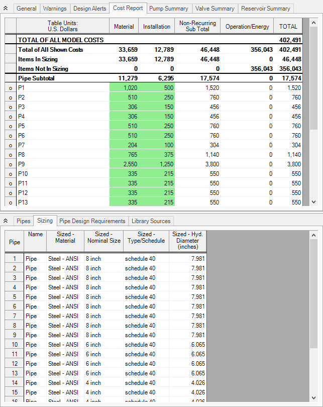
Now load the FCV Initial Cost Sizing scenario and go to the Sizing window to the Sizing Objective panel. Under Options to Minimize Monetary Cost, choose Size for Initial Cost, Show Energy Costs. The scenario is now ready to be run.
Run the model, then click the Output button once the automated sizing is completed.
After sizing the model for Initial Cost, the total cost over 10 years is now calculated as
Although this sized system uses much large pipe sizes, and therefore increased material and installation cost, than the initial design (4-8 inch versus only 4 inch), the savings comes from a the sized pump requiring much less power to operate. In one short simulation, the system was sized to meet all design requirements and reduce the cost by close to $1 million.
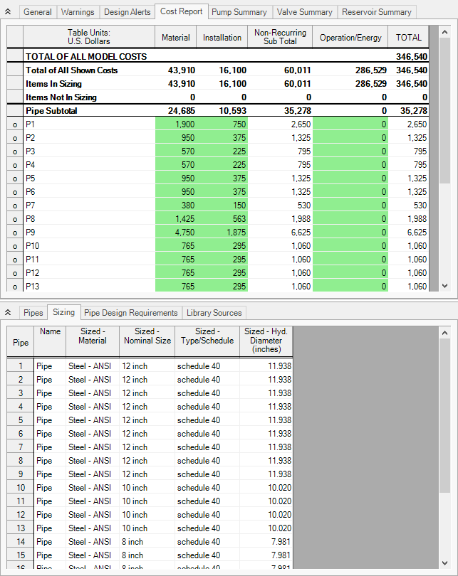
Step 10. Size the system based on lifetime cost
In the Scenario Manager on the Quick Access Panel, make a child scenario from the Base Scenario named FCV Life Cycle Sizing. Load then run this scenario.
On the Output tab in the Cost Report, it can be seen that the total cost for this case is
Step 11. Choose an Actual Pump for the System
Create a child scenario from the FCV Life Cycle Sizing scenario, and name the new scenario FCV Real Pump. We will now need to update the Pumps and Control Valve with the settings for the proposed system. Load the new FCV Real Pump scenario using the Scenario Manager, then make the following changes:
-
For each of the pumps open the Pump Properties window and select Pump 2000 gal/min Real from the Library Jct list. This will copy the Pump Curve data into the pump. Click OK. Make sure to do the same for the second pump.
-
Open the Control Valve and change the Valve Type to Flow Control (FCV) with a Volumetric Flow Rate of 2000 gal/min. Click OK
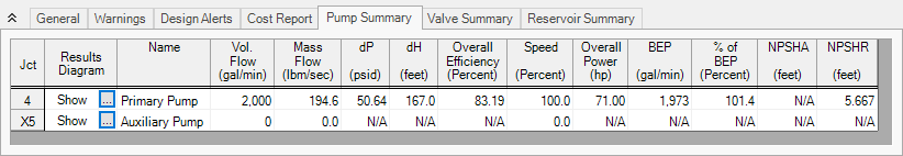
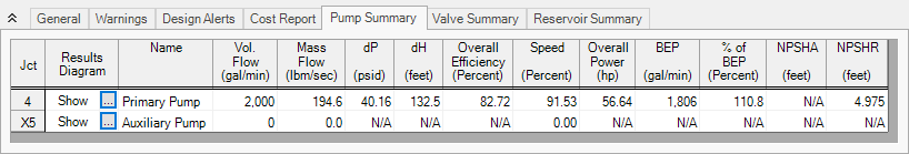
The model should now be ready for analysis. Run the model once more and go to the Output window to review the results, as can be seen in Figure 8 and Figure 9. Note that this scenario does take a bit longer to run than the sizing scenario. With data for the actual pump, the automated sizing finds a slightly more efficient design for the Life Cycle cost analysis by using 6 inch lines at some of the generators rather than 8 inch lines, which provides approximately $10,000 reduction in cost from the sizing scenario. Note that the Overall Efficiency is 83% for the real pump compared to the assumed 80% of the original sizing pump.

Step 12. Compare Cost Using a VFD Pump
As a final step we will compare an alternate VFD model for the pump to analyze the cost savings which can be achieved by using a VFD instead of using a flow control valve. To start, make an additional child scenario from the FCV Life Cycle Sizing scenario, and name it VFD Pump. Complete the following steps to update the model:
-
Go to the Workspace. For each of the pumps, open the Pump Properties window and choose the Pump 2000 gal/min VFD Real pump from the Library Jct list. Click OK
-
Open the Control Valve Properties window. On the Optional tab set the Special Condition to Fully Open - No Control. Click OK.
-
Go to the Sizing window, and go to the Design Requirements panel. For the Control Valve uncheck the box for the minimum pressure drop requirement, since the control valve is not active.
-
Navigate to the Assign Cost Libraries panel. We will need to represent the additional Material/Installation costs for the VFD, so change the Libraries to All so that all libraries will be applied for each of the pumps.
The changes for this scenario should now be complete. Run the model once more and go to the Output window to review the results. With the VFD Pump being used, the sizing for the pipes is actually the same as the FCV Life Cycle Sizing scenario. However, the cost is significantly decreased to
Summary
A summary of the total costs for each of the scenarios can be seen in Table 1. It can be seen from the table that this particular system over its 10 year life span is heavily weighted towards operational costs; as the operational costs are further decreased the overall cost for the system decreases, even though the initial costs may be increased.
Table 1: Summary of Automated Sizing Results for Lube Oil System in thousands of dollars
| Life Cycle Cost (U.S. Dollars) | Feasible? | Material | Installation | Total Non-Recurring | Operation/Energy | Total Life Cycle |
|---|---|---|---|---|---|---|
| Calculate Costs, Do Not Size | No | 70,387 | 23,722 | 94,109 | 1,273,892 | 1,368,001 |
| FCV Initial Cost Sizing | Yes | 33,659 | 12,789 | 46,448 | 356,043 | 402,491 |
| FCV Life Cycle Sizing | Yes | 43,910 | 16,100 | 60,011 | 286,529 | 346,540 |
| FCV Real Pump | Yes | 42,489 | 15,813 | 58,302 | 278,154 | 336,455 |
| VFD Pump | Yes | 55,293 | 19,306 | 74,599 | 221,872 | 296,471 |


