Optional Input
Initial Flow Rate Guess
The Initial Flow Guess for a pipe can be specified. An appropriate initial guess can decrease the number of iterations required to arrive at a converged solution. This initial guess will only affect the steady-state solution process.
The Solver generates initial guesses on its own, which is usually sufficient to get the Solver going in the right direction so a converged solution results. If this is not the case, user defined guesses can help obtain a solution.
Stagnant Region Steady-State Pressure
You can specify a reference pressure in a pipe that will be closed during steady-state which will be used for the transient simulation. Only specify one pressure per stagnant region or you will receive an error stating there is more than one stagnant pressure defined. A single stagnant pressure will allow Impulse to calculate the pressures in the region with hydrostatic pressure differences due to elevation change being taken into account.
Pipe Line Size and Color
Each pipe may have its line size and color changed from the defaults configured in Workspace Options.
Workspace Display
By default, only the pipe number is displayed on the Workspace. In addition to this, the pipe name, nominal size, and type/schedule can be displayed.
Design Factors
A design factor can be used to add safety margins into the hydraulic analysis. For pipes, two design factors exist:
-
Pipe Friction: friction factor is multiplied by the design factor assigned to the pipe.
-
Pipe Fittings & Losses: total loss factor (K factor or Equivalent Lengths) is multiplied by the design factor assigned to the pipe.
Support for Partially Full Pipe
There is checkbox which indicates the pipe supports partially full pipe calculations. This means partially full along the axial direction (length), as opposed to partially full along the radial direction (radius). This function only works for pipes that have a slope, and when the pipe is partially full it drains from the end with the higher elevation.
If this feature is not selected, the pipe will always be assumed to be liquid full. Selecting this feature implies that one end of the pipe is connected to a junction at its higher elevation endpoint which allows gas to flow in, thus allowing the pipe to drain.
If the option is selected, and the entry is 100%, it means the pipe is initially 100% full, but can drain if backflow occurs at the high elevation endpoint. The percent full can also be set to something less than 100%. In this case, the pipe is assumed to be partially full initially. This is only valid when the steady-state condition for the pipe is such that there is no flow, since if there were flow in that pipe during steady-state, the pipe would not be partially full.
This feature only works with pipes which connect to a air valve, spray discharge, assigned pressure or exit valve junction at the high elevation end. When selected, the predicted level of the liquid surface and other related parameters can be graphed in the Graph Results window. When pipes can be partially full, more accurate predictions result when the pipe is modeled with more sections. At least two sections should be used, and more if possible. This is because Impulse will model each section in the pipe as either completely liquid full or empty. Therefore, more sections in the partially full pipe will allow Impulse to more precisely determine the liquid level.
Parallel Pipes
A single pipe object can be specified as a number of parallel pipes. When multiple pipes are defined, the parameters in the pipe properties window represent only one of the parallel pipes.
The inlet and exit elevations of a pipe are equal to the elevations of the upstream and downstream junctions. The pipe elevation is assumed to vary linearly between the junctions. In other words, the pipe is assumed to be perfectly straight.
Modeling a large number of elevation changes with straight pipes would require a large number of junctions, as shown below:
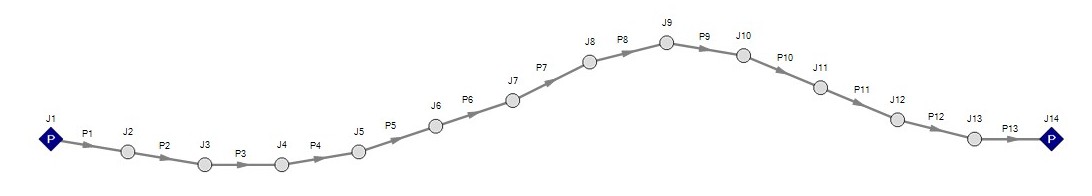
Figure 1: Accounting for elevation changes with many pipes and junctions
This is tedious and not required for overall hydraulic calculations - only the elevation change across a (fluid full) pipe is needed. However, intermediate pressure results along the pipe will be affected.
For example, Figure 1 shows elevation extremes both lower and higher than the elevations at the ends of the pipeline. Low points may exceed maximum allowable pressures, and high points could drop below vapor pressure. If this is modeled as a single straight pipe these issues would not be easily identified. In fact, if these pipes were replaced with a single pipe it would show no elevation change at all!
Instead of using a large number of pipes, these effects can be accounted for in a single pipe using intermediate pipe elevation feature.
With length defined, check Use Intermediate Pipe Elevations, choose the elevation units, the number of intermediate elevations (a 2 segment pipe has 1 intermediate elevation), and whether the entered values are Point to Point or Length Along Pipe.
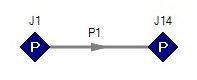
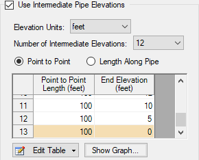
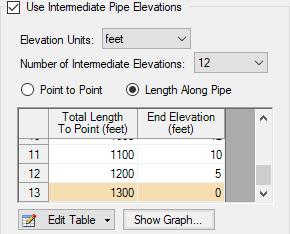
Figure 2: Intermediate Elevations - Identical Profiles defined with both methods
AFT Impulse will ensure the total length matches the length on the Pipe Model tab. It does so by fixing the length of the final section to the difference between the sum of the lengths in the table and the actual length entered by the user. The end elevation is also fixed by the downstream junction. If the user later modifies the downstream junction elevation, the pipe’s final elevation section will be automatically updated. The maximum number of rows available in this table can be changed in User Options.
After the intermediate elevations have been entered, a graph showing the data can be displayed. Below is the profile graph of the pipe described above.
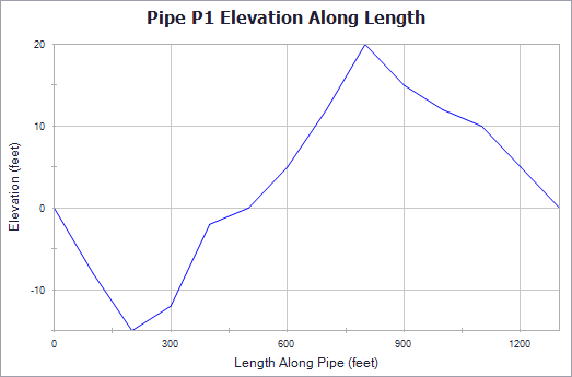
Figure 3: Intermediate Elevation Graph
Related Topics
Pressure Drop in Pipes - Detailed Discussion
Pipe X segment length Y is shorter than the elevation change
Related Blogs


