Four Quadrant Dimensional Reference Point
As described in Four Quadrant Data Sets, data specific to a given pump is rarely available. Instead, four quadrant test data from a different pump with similar specific speed is commonly used as an estimation. Because the Suter method stores the four quadrant data in dimensionless form, the data must be made dimensional.
As described in Four Quadrant Model Overview, the data is made dimensionless by dividing each parameter by some reference value:

To obtain the original values, the dimensionless parameters can simply be multiplied by the original reference values. This only works to recreate the values for the original pump - the pump of interest (the "similar" pump) - may be of a similar specific speed, but of different size. In this case, different values will be used in dimensionalizing the data. These four reference values are referred to as the Four Quadrant Dimensional Reference Point.
Multiple Choices for a Dimensional Reference Point (DRP)
Traditionally, the Dimensional Reference Point used to create the dimensionless data will be the rated conditions at the pump's Best Efficiency Point. Applying these same rated conditions to the dimensionless data will fully recover the original data. Due to the nature of using similar four quadrant data sets to estimate behavior, the DRP used to "unpack" the data will almost certainly be different than the DRP originally used in its creation. There are a couple of reasons for this.
First, the tested pump may have identical specific speed - and perhaps even identical behavior - to the pump under analysis, yet still have a different pump curve. This is because a pumps of different size but identical construction will behave in a similar way. This is at the root of the homologous pump laws, which are used to derive the affinity laws. The data from one pump can be made dimensionless with that pump's DRP, and made dimensional for the other pump with the other pump's DRP. If these two pumps are truly homologous, then the actual, dimensional behavior of the second pump will be fully and accurately represented. Of course, two pumps are very unlikely to be truly homologous and therefore this process will introduce some error.
Second, it is not necessarily required to use the same "type" of DRP for unpacking the data. By default, AFT Impulse uses the rated conditions at Best Efficiency Point. Also available is the option to use the Steady-State Operating Point. Both of these options are estimations, and both have certain advantages and disadvantages.
Note: The choice of Dimensional Reference Point should not be taken lightly. The choice can have significant impacts on the results of a transient simulation, potentially indicating a system is safe when significant transient cavitation could occur, or perhaps indicating that cavitation will occur when it may in fact be unlikely. (Walters, Lang, and Miller, 2018 Walters, T. W., Lang S. A., and Miller D. O., "Unappreciated Challenges in Applying Four Quadrant Pump Data to Waterhammer Simulation, Part 1: Fundamentals", Proc. 13th International Conference on Pressure Surges, BHR Group, Bordeaux, France, November 2018. )
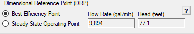
Figure 1: Specification of DRP in AFT Impulse.
Using Best Efficiency Point as the DRP
AFT Impulse can calculate the pump's rated parameters at the Best Efficiency Point (BEP) when the Standard Pump Curve is defined with the required efficiency/power data and a rated speed. With this option selected, these parameters become the DRP.
As mentioned, the Four Quadrant Data Set in use was likely created with the BEP of the test pump as the DRP. If the two pumps are similar, it is therefore reasonable to use the BEP of the new pump as the DRP. If the Four Quadrant Data Set is well matched, the resulting Four Quadrant Curves will closely match the Standard Pump Curve. If the curves appear to be well matched in the Normal Pumping Zone - having similar shape, shutoff, and runout head - it is likely, although not guaranteed, that the Four Quadrant Curve is reasonably accurate under reverse flow and speed conditions as well.
Because the BEP of the pump is an unchanging value, the same Four Quadrant Curve will always be generated regardless of where the pump is running on its curve. This means that if the pump is not running exactly at BEP, even a well matched Four Quadrant Data Set will likely not agree exactly with the Standard Pump Curve. A "jump" from one curve to another can not be allowed during a transient simulation as this would induce an Artificial Transient. To avoid this, the Standard Pump Curve is not used in simulation when BEP is selected as the DRP. The Standard Pump Curve is only used for the purpose of generating the required DRP.
This means that the steady-state results will not agree with the the Standard Pump Curve unless the data was perfectly matched. This is an area where the estimation begins to have an impact. If the steady-state results are of critical importance in the transient simulation this may be unacceptable. Typically, variations in steady-state behavior are acceptable when analyzing a transient event, as the magnitude of pressure and velocity changes from transient events far outweigh small steady-state differences.
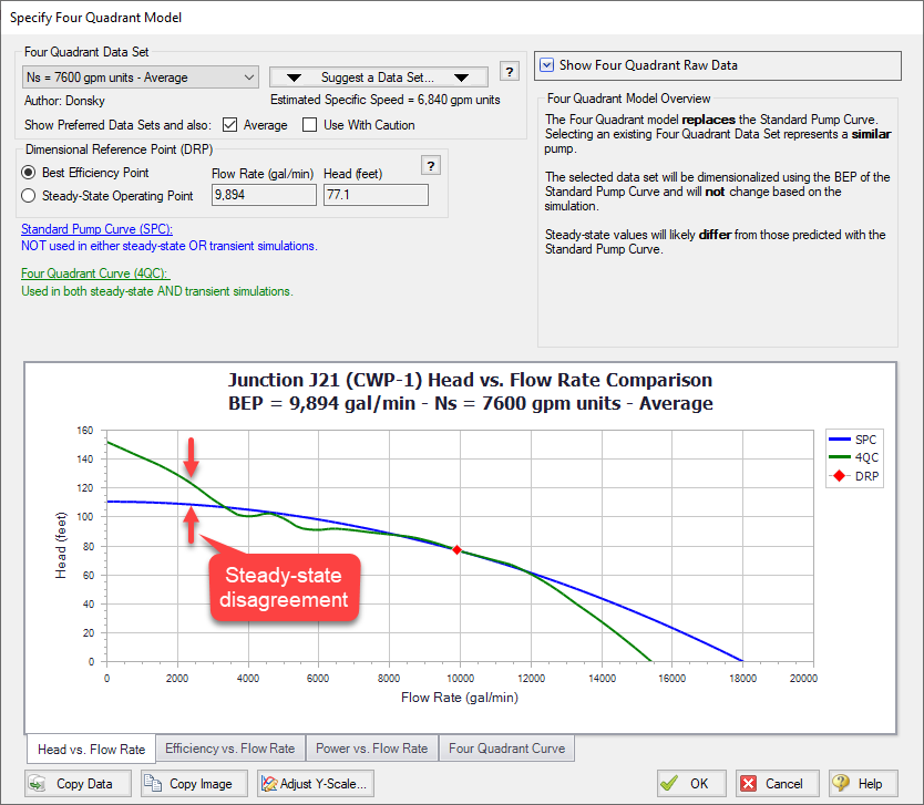
Figure 2: Using Best Efficiency Point as the DRP. The Four Quadrant Curve is static and disagrees in some areas with the Standard Pump Curve. However, the curve matches reasonably, especially near BEP.
Using Steady-State Operating Point as the DRP
If the decrease in accuracy of the steady-state results is unacceptable, it is possible to use the Standard Pump Curve in the steady-state simulation to obtain accurate results. If this is done, another approach must be taken to avoid "jumping" curves and inducing an Artificial Transient. Instead of using the BEP, it is possible to use the Steady-State Operating Point as determined directly with the Standard Pump Curve during the steady-state simulation.
When dimensionalizing the Four Quadrant Data Set with the DRP, the resulting Four Quadrant Curves will be forced to pass through the DRP. In other words, the Standard Pump Curve and the Four Quadrant Curve will be made to intersect exactly where the pump is operating. This has the effect of eliminating any Artificial Transient, while allowing the steady-state simulation to use one curve (the Standard Pump Curve) and the transient simulation to use a different curve (the Four Quadrant Curve).
Keep in mind that the method itself is identical - only the DRP used to carry it out has changed. In fact, if the pump happened to be operating exactly at BEP, the two methods would be completely identical.
Unlike the BEP option, the generated Four Quadrant Curve will change based on where the pump is running on its curve. In effect, the original Four Quadrant Data Set is being distorted to match at the steady-state condition. This means that despite the increase in steady-state accuracy we are not able to get away from the fact that this is still an estimation. By reducing error in one area, it has been amplified in another.
What does it mean to say the curve has been distorted? Because the Four Quadrant Data Set represents a certain "character" of pump, the overall shape and trends of the data cannot be changed. By using a different DRP, the data is instead "shifted" as necessary in the appropriate directions. For example, if the Steady-State Operating Point is calculated to have lower flow and higher head than the BEP, the entire Four Quadrant data set will be compressed in the "flow direction" and stretched in the "head direction" to force the original reference point to meet the new reference point.
If the pump is operating far from BEP, this can potentially result in severe distortion of the Four Quadrant Pump Curve. In such cases, the pump behavior is accurate during the steady-state simulation, but may differ wildly from the Standard Pump Curve under different flow conditions.
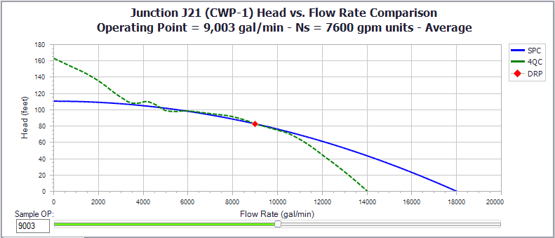
Figure 3: Using a Sample Steady-State Operating Point as the DRP for the same Standard Pump Curve shown in Figure 2. The point is near BEP so the curve still matches reasonably well.
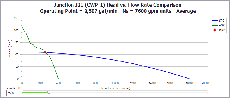
Figure 4: Using a Sample Steady-State Operating Point far from BEP introduces significant distortion. The curves still match at the DRP, but the differences are severe at other flows.
Which DRP should I use?
The question of which point should be used may be obvious, but the answer is not. The best approach is to try and ensure that the Four Quadrant Curve reasonable matches the Standard Pump Curve for the expected range of operation.
If it is not clear which option is better, it is recommended to do a sensitivity analysis and run cases of the model with both options. Note that because both methods are estimations, this does not "bound" the possible solutions. Instead, it will give some idea of how impactful the choice is. Large differences in simulation results should encourage close attention and high safety factors. See the Four Quadrant Data Set Selection topic for more details.


