Four Quadrant Model Overview
Four Quadrants of Operation
To accurately model a pump undergoing reverse flow or speed, or pumps past the runout flow, test data for those regions must be available. In certain cases rough approximations can be made without this data, but as with any model, good results require good data that reflect the actual characteristics.
Turbomachines can operate at any flow or speed, positive or negative. The speed-flow plane thus creates four quadrants - hence the name Four Quadrant.

Figure 1: The speed-flow plane, showing the four possible quadrants of operation.
At any given speed and flow combination, there is an associated head and torque. Any given turbomachine must operate on these surfaces of points defined by head-speed-flow and torque-speed-flow in steady-state.
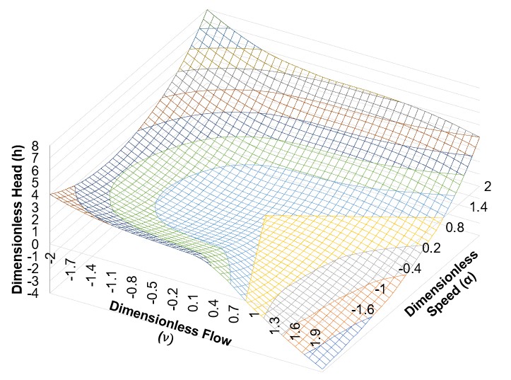
Figure 2: Relationship of head to flow and speed over all four quadrants
Such a surface is usually presented as a contour plot, with curves of constant head and torque drawn on a 2 dimensional speed-flow diagram.
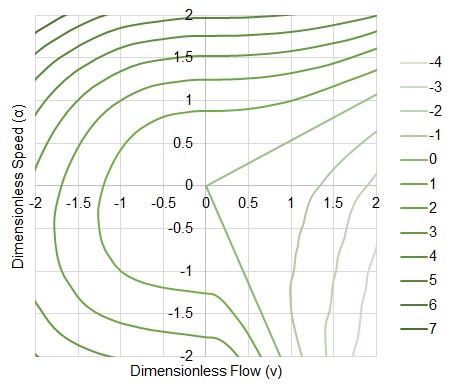
Figure 3: Contour plot showing lines of constant head. Same data as Figure 2.
Similar data for torque can be presented on the same plot, commonly referred to as a Karman-Knapp Circle Diagram.
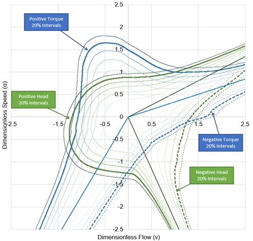
Figure 4: Constant contours of torque and head for a particular turbomachine. This is the same pump as Figures 2 & 3, but with different contours included.
This is the data required to model a turbomachine under reverse flow and speed. But how do we apply it? And what simplifications can be made?
Simplifying the Data with the Affinity Laws
A real turbomachine has characteristics unique to certain operating speeds or flows. For example, a very high flow or speed may induce transient cavitation, severely impacting head generated. On the other end of operation, a very low speed will be more impacted by friction of the various rotating components. If the flow is low enough, it will become laminar, changing the behavior of the fluid dramatically.
To fully account for these real effects, a simulation would need actual data for every possible situation. In other words, a set of curves such as that shown in Figure 4 would be the minimum data entry. Clearly, this would be an enormous amount of data to enter, if it was even possible to acquire. Fortunately, these effects - although real - do not need to be considered for the vast majority of pump studies.
To greatly simplify the data required, the pump can be considered as completely homologous - meaning that the affinity laws apply for all speeds, flows, heads, and torques. This means that instead of a large collection of curves, only a handful of curves are required, as the others can be appropriately "scaled" from the source curve.
In fact, the curves shown in the figures above represent exactly this scaling - they do not represent raw measurements for each combination of speed and flow. Instead, most of the contours were generated using the relationships defined by the affinity laws, with only full speed (positive and negative) values being measured, as represented by the bold contours.
Applying the Data in Numerical Simulation
It would be possible to use the raw data defined by a set of curves such as that shown above directly in a numerical simulation. One approach used in the early days was to store many curves in familiar forms such as head vs flow and torque vs flow at a variety of speeds. This approach, while valid, can pose great difficultly in computational analysis because every parameter - head, torque, speed, and flow - can become zero at any point during the simulation. Determining which curves to use and handling zero values dynamically is difficult.
An alternative method, proposed by Suter, 1966 Suter, P., Representation of Pump Characteristics for Calculation of Waterhammer, Sultzer Technical Review Research Issue, pp. 45-48, 1966. , involves transforming the data into a different coordinate system such that the values of numerical interest never become zero. This method, used by AFT Impulse, is commonly referred to as the "Suter Method."
Before proceeding with the transformation, the measured data from a particular turbomachine is made dimensionless by dividing through by a Dimensional Reference Point. It should be noted that these rated values are traditionally considered to be the rated values at the Best Efficiency Point. However, alternative references can be used in some situations.
Because there are four parameters, four reference values are required to make the data dimensionless, like the data presented in Figure 4 above.

where
h = Dimensionless head
H = Dimensional head
β = Dimensionless torque
T = Dimensional torque
α = Dimensionless speed (note that α is commonly used to denote angular acceleration. To maintain consistency with the literature, this represents the dimensionless speed here)
N = Dimensional speed
ν = Dimensionless flow
Q = Dimensional flow
The data can now be transformed into a more useful coordinate system. For any given point on one of the head curves (as an example), there is a specific value of speed, flow, and head. Drawing a line from the origin to this point creates an angle to the exiting axis.
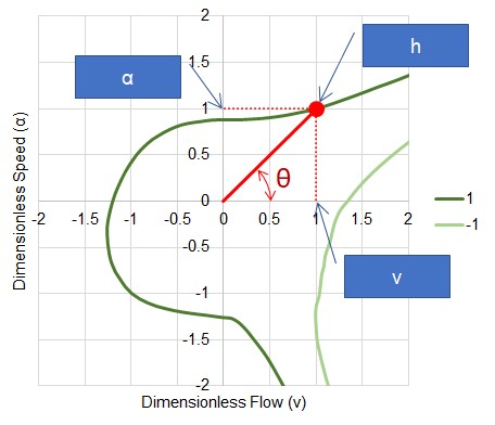
Figure 5: Transforming the data
The angle is simply defined with trigonometry:

or in some definitions:

To define the point itself, the following equations are used for head and torque, respectively:


For the point shown in Figure 5, FH evaluates to 0.5, with a Θ of 45 degrees. Applying this transformation to all of the data in the speed-flow plane, we can construct values of FH and FB for all Θ. In other words, FH and FB are continuous functions of Θ.
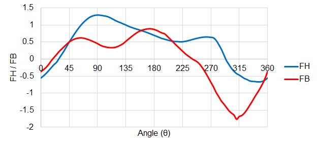
Figure 6: FH and FB values for all Θ. This is still representing the same data as all previous Figures.
By reversing the transformation, data in a standard form such as head vs flow can be recovered fully.
Note: All of the above example Figures represent the Ns = 0.66 (1800 gpm units) data set, available in AFT Impulse. For this reason Figures 2 - 4 do not show divergence from the affinity laws (it is not raw data, but back-calculated from the data shown in Figure 6).


