Transient Sensitivity Analysis Tutorial
AFT xStream requires a large number of inputs to be defined in order to run a transient simulation. Many of those inputs directly affect the transient simulation results, and it is important for users to carefully evaluate that effect. This tutorial will focus specifically on three parameters: the Minimum Number of Sections per Pipe defined in the Sectioning Panel, the Fluid Property model used, and the estimated Maximum Mach Number in Pipe value.
We will use the model shown below in Figure 1 of a system with an abrupt stoppage of flow at a Turbine Shutoff Valve (TSV) to indicate how a user might analyze results and refine these inputs over subsequent runs. To help quantify how these parameters impact the transient simulation results, we will look at transient forces in the system, using a Difference Force Set applied to each pipe. Please note that this tutorial is not meant to be an exact step-by-step procedure to follow, but is instead meant to be a general guideline to help the user better understand how to evaluate xStream results.
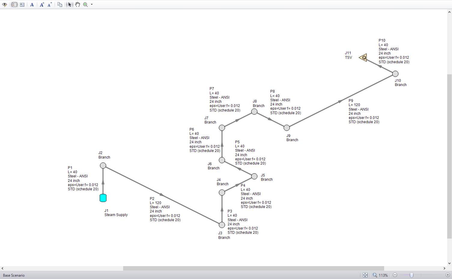
Figure 1: Layout of Tutorial Example
Baseline Results
We must start our sensitivity analysis by determining some baseline results for the system. The first run of the model uses standard settings for all inputs: AFT Standard Steam using the Three-Parameter method, the default Maximum Pipe Mach Number During Transient of 1, and a Minimum Number of Sections per Pipe of 10. Force results from this run for Pipes 2,3,8, and 9 are shown below in Figure 2.
Pipes P2 and P9 see the largest transient forces in this model, mostly because P2 and P9 are 120 ft long with the other pipes in the system are 40 ft long. Transient forces are caused by the presence of transient waves with some pressure differential across them traveling through the system. A longer pipe which is long enough to contain the entire wavefront will see a larger pressure differential across it than a shorter pipe which only ever sees a portion of the wavefront. Thus, longer pipes tend to see larger transient forces, with the maximum transient force seen when the entire wavefront is shorter than the pipe length.
We can also see that P2 experiences a significantly higher maximum transient force than P9 even though they have the same length. This difference is due to wave coalescence (or wave steepening). A wave moving through a gas raises the local temperature, in turn raising the local sonic velocity. The temperature and sonic velocity behind the wavefront is thus higher than that ahead of the wavefront, meaning the back of the wavefront can have a higher wave velocity (V+a) than the front of the wavefront. As the wave travels, the back of the wavefront will catch up to the front of the wavefront, steepening the wave until a shock wave is formed.
In this example, P9 is closer to the transient event at J11, and the wavefront is still relatively dispersed. However, the wavefront has steepened by the time it reaches P2, meaning more of the wavefront can fit in P2 and a larger transient force is seen.
This tutorial will focus on the transient force results from P2, as they are the largest magnitude forces in the model.
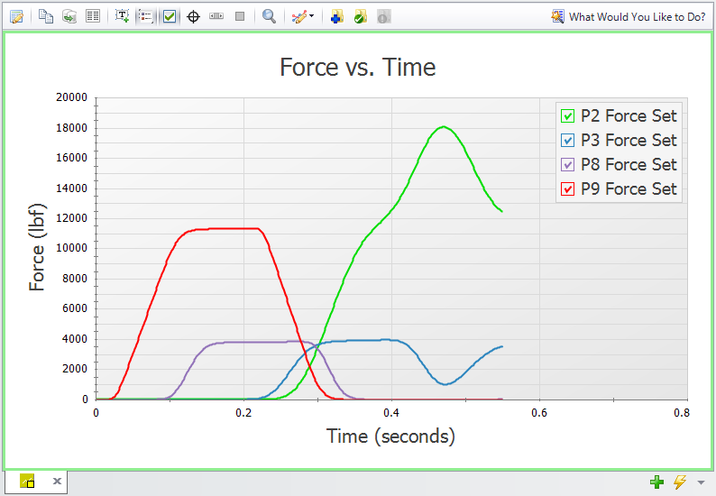
Figure 2: Force Results for AFT Standard, 10 Minimum Sections, Standard Maximum Mach Number in Pipe
Minimum Number of Sections Per Pipe
The first parameter for our sensitivity analysis is the Minimum Number of Sections Per Pipe. The baseline scenario used a minimum of 10 sections, and we will also run scenarios with a minimum of 50 and 100 sections. All other inputs are held constant, and results for the P2 Force Set are shown in Figure 3 below.
Comparing the 10 section and 50 section scenarios, the 50 section scenario gives a force that is
We now know that 50 sections is a good point to balance accuracy with run-time concerns.
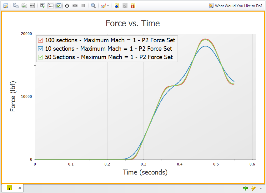
Figure 3: Effect of Sectioning on Forces
Fluid Property Model
The next parameter for our sensitivity analysis is the Fluid Property Model. The baseline scenario used AFT Standard Steam with the Three-Parameter equation of state, and we will also run scenarios using AFT Standard Steam with the Redlich-Kwong equation of state, Chempak Steam, NIST REFPROP Steam, and ASME Steam. All other inputs are held constant, and results for the P2 Force Set are shown in Figure 4 below.
The results shown in Figure 4 below show that the Fluid Property Model can have a substantial impact on results. The largest difference in results is between the Chempak and Redlich-Kwong results, with an absolute difference of
The observed difference in transient force magnitude for various Fluid Property models forces us to evaluate which model is best suited for this system.The Redlich-Kwong and Three-Parameter equations of state were developed for light, non-polar molecules - hydrocarbons in particular. Water (or steam, in xStream) is a relatively light molecule which is highly polar, meaning the accuracy of those Fluid Property models may be reduced when evaluating the steam in this system. Chempak has an increased accuracy from the AFT Standard Steam models, and gives force results which are substantially higher. It is difficult to say how reliable the Chempak results are until we compare them against other models.
Finally, the scenarios using NIST REFPROP Steam and ASME Steam give effectively identical results, and the source for each model (NIST and ASME, respectively) is highly reliable. We can thus say that these results are the most reliable results, and they should be used for subsequent runs of our model. The only distinguishing factor between these two Fluid Property Models is the model run time, where the NIST REFPROP model will run significantly faster than the ASME Steam model. See the Fluid Property Model example for more information on this topic.
To learn more about the strengths and weaknesses of each fluid property library, visit the Fluid panel topic. Note that while the NIST REFPROP and ASME Steam models may offer improved accuracy, the AFT Standard fluid models run significantly faster. Users should always use the AFT Standard fluid models for initial runs as the xStream model is gradually refined.
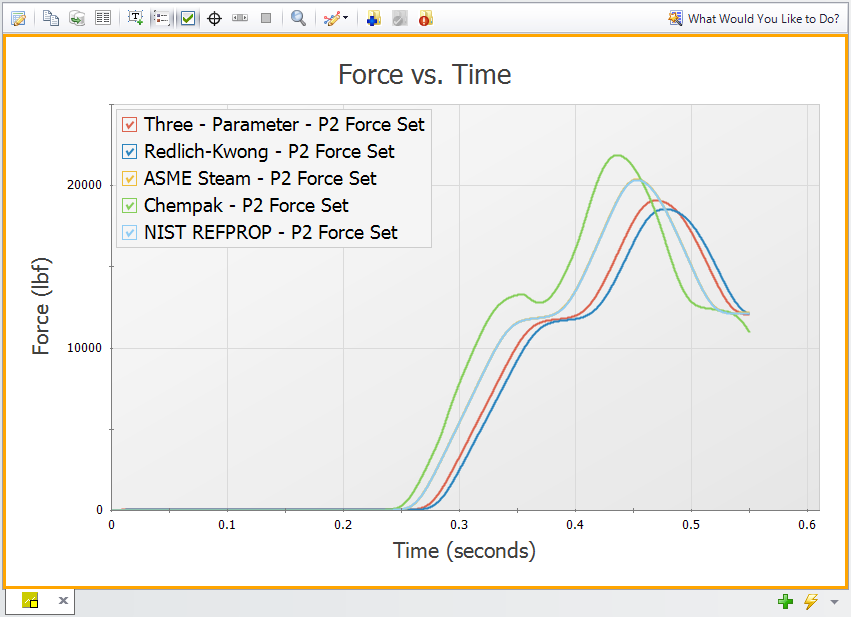
Figure 4: Effect of library on Forces (minimum 50 sections used in each pipe, ASME Steam has indistinguishable differences from NIST REFPROP and thus cannot be seen in this figure)
Effect of Maximum Pipe Mach Number During Transient
The last parameter for our sensitivity analysis is the Maximum Pipe Mach Number During Transient, defined in the Pipe Sectioning and Output panel. The MOC grid size is determined by the wave velocity (V+a), using the maximum estimated sonic velocity. This maximum sonic velocity is in turn a function of the Estimated Maximum Pipe Mach Number During Transient and the Estimated Maximum Pipe Temperature During Transient input parameters. Refining the estimated maximum sonic velocity can improve the accuracy of our results by reducing the amount of interpolation necessary while performing the MOC calculations.
The results for our model when using a minimum of 10 sections and ASME Steam show a Maximum Mach Number of 0.06, seen in Figure 5 below. Reducing the Estimated Maximum Pipe Mach Number During Transient from the default value of 1 to a value closer to 0.06 may improve our results.
Figure 6 below compares transient force results with Estimated Max Mach Numbers of 1, 0.5, and 0.1. A scenario with 50 sections is included as a reference for what the expected results are, based on our previous analysis of how sectioning affects results. We can see that better estimates of the Max Mach Number for the transient simulation bring the results with 10 sections closer towards the 50 section reference results. However, better estimates for the Max Mach Number are unable to make the 10 section results match the 50 section results, indicating that the user should use the Estimated Max Mach Number parameter to compliment adding additional sections rather than to replace adding additional sections.
Caution: Never define the Estimated Maximum Pipe Mach Number During Transient lower than the value observed in the system! An estimate lower than the actual value will force the MOC calculations to extrapolate, which can add significant instability and uncertainty to the results. Output which shows that the specified maximum Mach number was exceeded should be disregarded, and a better Estimated maximum Pipe Mach Number During Transient should be defined.
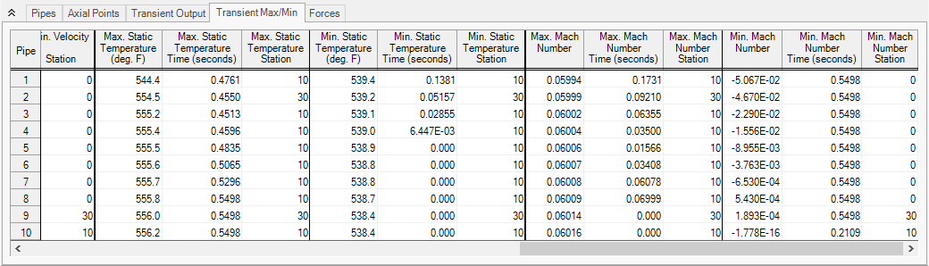
Figure 5: Maximum Mach Number obtained from 10 Sections, ASME Steam, Maximum Mach Number of 1
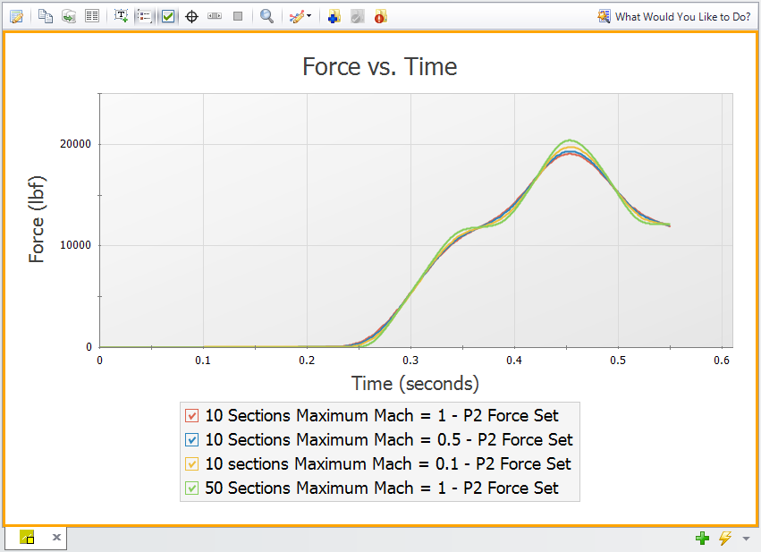
Figure 6: Effect of Maximum Pipe Mach Number During Transient on Forces
Comparing Initial and Optimized Inputs
Our sensitivity analysis on Minimum Number of Sections Per Pipe, Fluid Property Model, and Estimated Maximum Mach Number in Pipe showed what inputs to use for this model. Figure 7 below compares the initial results (10 minimum sections, AFT Standard Steam with the Three-Parameter equation of state, and a Max Mach Number of 1) against the final results (50 minimum sections, ASME Steam, and a Max Mach Number of 0.1). These transient force results show a different timing of the transient waves, a different shape of the wavefront, and a difference in the maximum force magnitude of
These differences help show the importance of gradually refining the model input parameters. Initial runs should be performed with default or more simple options which have faster run times as the user starts to understand the system. Then, the user should refine the inputs for more advanced parameters to reduce the uncertainty in their results.
Note that some systems may be more sensitive or less sensitive to the three parameters considered in this tutorial. The user should follow these steps on their own system and use their engineering judgment to determine the best model inputs.
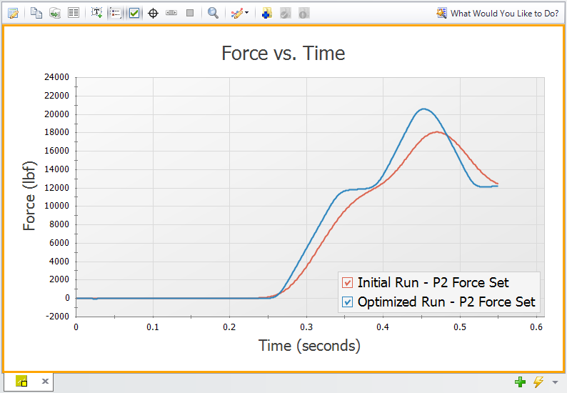
Figure 7: Initial Run vs Modified Run
Related Topics
Pipe Sectioning - Introduction to Method of Characteristics
Pipe Sectioning and Output Group
Interpreting Transient Results
Related Examples


