Transient Result Accuracy
Modeling transient, compressible flow in a pipe network is an inherently imprecise endeavor. Individually modeling transient flow, compressible flow, or transient compressible flow in a single pipe can be done to a high degree of precision, but the practical application of all three factors forces limiting assumptions to be made. AFT xStream is no exception. The methods it employs start from three fundamental equations: conservation of mass, momentum, and energy. However, solving those equations on a practical scale requires several limiting assumptions that introduce some amount of error into the results. The derivation process and these assumptions are discussed in detail in the Transient Theory section.
As the user analyzes and interprets their transient results, it is important they keep in mind how the assumptions behind the MOC solution introduce error, how to gauge that error, and how to reduce that error.
Sources of Error
The MOC solution process includes multiple assumptions, with two primary assumptions being made. First, flow parameters are assumed to vary linearly between computation stations, allowing linear interpolation to be performed. Second, fluid properties are assumed to be constant while integrating along characteristic lines, allowing those integrals to be solved directly. In effect, this means that fluid properties are only updated once per time step, with their change over time assumed to be linear.
The nature of the MOC solution forces both assumptions to be made. The MOC solution requires that the time step at each location in the system be uniform, meaning the section length must also be held constant. In an incompressible fluid system such as an AFT Impulse model, these assumptions introduce a minimal amount of error. However, in a compressible fluid system such as an AFT xStream model, these assumptions introduce a potentially significant amount of error as the compressible nature of a gas means flow parameters and fluid properties are changing continuously in time and space.
Users of AFT Arrow may be familiar with how Arrow captures the continuously changing nature of compressible flow. Arrow calculates results at intervals along a pipe which are adjusted based on the change in Mach number, thus the compressible flow effects along a whole pipe are accurately captured even though properties between computation stations are assumed to change linearly.
xStream however, does not have the ability to adjust the locations at which properties are calculated to be specific for an individual pipe. Section lengths must be held constant across all pipes in a system. Adjusting the location of computation stations along a single pipe would require the time step to change across the simulation, which in turn could cause time to run faster in some parts of the system than in others.
Gauging Error
These assumptions have the major implication that mass and energy may not be perfectly conserved along the length of a pipe. The error introduced by these assumptions increases as the compressible flow effects become more pronounced. At low Mach numbers, mass and energy can be almost perfectly conserved, while near the sonic velocity, potentially significant amounts of mass and energy may escape the system.
Users can gauge this error in their system via two means. The first is more quantitative and is performed for the user by xStream. Prior to implementing the MOC transient solver, xStream solves the system once using the same computational methods as used by AFT Arrow, and once by running the MOC solution without any transient events to determine the MOC Steady Solution.
The mass and energy loss along a pipe in the MOC Steady Solution can then be quantified. The mass and energy flow out of each pipe are subtracted from the mass and energy flow into each pipe. In a nominally steady-state system, the difference should be zero. However, the assumptions behind the MOC solution mean this difference may not be zero. The steady-state error is reported in the Solution Progress window, and the simulation process will be halted if the steady-state error exceeds the allowable set points. Figure 1 below, shows what that reported error and halted solution looks like. It is important to note that this quantitative approach to gauging error is only valid for a steady-state system. A transient system will inherently see differences in inlet and outlet mass and energy flows as waves travel along each pipe.
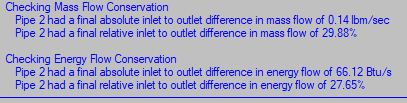
Figure 1: Solution Progress window showing an example model with high mass and energy conservation error
The second approach users can employ to gauge the error in their systems is more qualitative and must be performed by the user. Flow parameters and fluid properties change more rapidly in time and space at higher Mach numbers than they do at lower Mach numbers. Thus, in a system which sees high velocity or sonic choking either in steady state or during the transient simulation, users can expect to see relatively large mass and energy losses compared to systems with low velocities throughout. While users cannot directly quantify those losses, they can expect to be more confident in the results determined by xStream at lower velocities.
Reducing Error
The best way to minimize the error associated with the assumptions by the MOC solution process is to increase the number of sections in each pipe, which also decreases the time step in the simulation. This approach is similar to how Arrow captures compressible flow effects in steady-state systems. By calculating system parameters more frequently, the assumptions the MOC solution process makes are violated to a lesser degree.
In the Sectioning panel of the Analysis Setup window, users define the minimum number of sections a pipe can have. Setting a minimum section number of 5 means the shortest pipe must have at least 5 sections. Increasing that number forces xStream to use smaller section lengths throughout the entire system.


