Animating Graph Results
Animating the results of a transient run is an extremely powerful way to understand how a complex system is behaving. While transient plots of fluid parameters over time at a given location are valuable and easy to interpret, they do not directly convey the most important aspect of a fluid transient event - how the pressure and flow waves propagate through a system and interact with one another. Animating the results of a transient simulation allows you to observe these effects directly. Animations can also be created for Multiple Scenarios.
Creating an Animated Graph
Since animations display information along a flow path, only Profile type graphs may be animated.
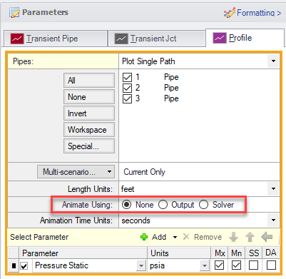
Figure 1: Options for animation under Profile type graphs in the Graph Results window
There are two ways to animate:
-
Animate Using Output - This option uses data saved to the transient output file. This option requires that the data for all stations in the path of interest was saved to the output file. This method is generally preferable as it is faster and allows the user to advance (or reverse) the animation to any given point. The only disadvantage of using Output for animation is that the required output files may be large.
-
Animate Using Solver - Instead of using saved data, this option re-runs the transient solver to generate the required data on the fly. This has the advantage of reducing output file size, but the animation must be displayed step-by-step and the transient calculation will be slower than reading from a file. For smaller models with graphs you do not intend to revisit, this may be acceptable. Generally, it is easier to save the data and use Animate Using Output. This option is not available for Multi-Scenario graphs.
Using an Animated Graph
Once the animated graph is created, it will look much like a normal Profile graph, but a few components have been added.
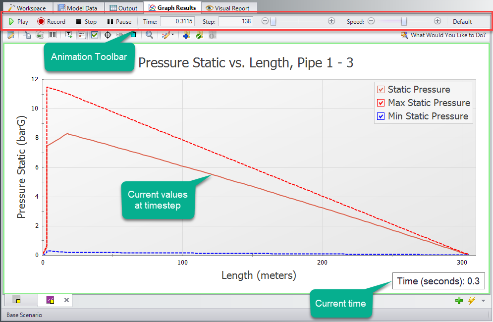
Figure 2: Components added to the Graph Results window when animating a Profile graph
The animation toolbar has several controls:
-
Play - Start the animation from the current time.
-
Record - Begin playing the animation from the current step, and when the playback is stopped, prompt the user to save an .mp4 video recording of the animation to file.
-
Stop - Halt the animation and reset the time to zero.
-
Pause - Pause the animation at the current time.
-
Time - The actual simulation time of the currently displayed data.
-
Step - The simulation step of the currently displayed data.
-
Time/Step slider - Seek for a certain point in the animation. If Animate Using Output was used, points later or earlier in the simulation can be navigated to directly.
-
Speed slider - Change the speed of the playback.
-
Default - Reset the speed to default.
By default, the graph will display the current values for the time step as well as the maximum and minimum profiles. These can be hidden or displayed in the graph Parameter selection area, like any other Profile graph. The Steady-State solution can be displayed, as well as applicable Design Alerts.
The Current Time box can be moved anywhere within the Graph area.
Using Animations to Interpret Behavior
There are many ways that animations are helpful in interpreting behavior. Below, we consider again the simple case of an instantaneous closure.
Like normal Profile graphs, multiple parameters can be displayed and animated as a single Graph List Item. The images below show the relationship between pressure and flow (velocity) for this case.
The animation showing the wave reflecting can be seen in Figure 5.
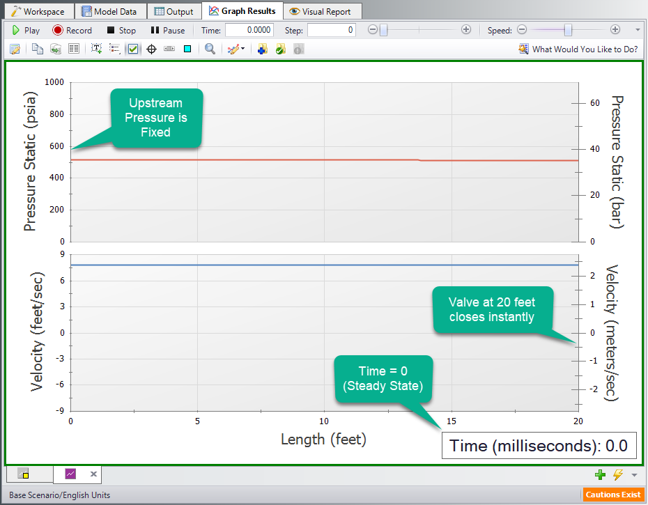
Figure 3: Animation showing steady-state (time step zero) results
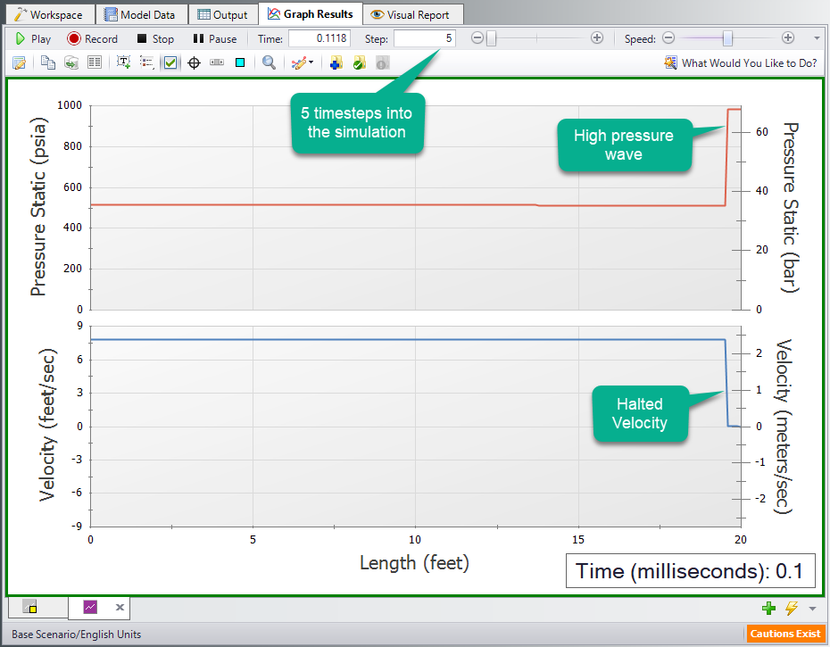
Figure 4: The instant closure of the valve halts the flow, causing a large rise in pressure
![]()
Figure 5: The movement of the wave within the pipe can be directly visualized


